From white paper to research plan

Chapter opening

A research plan for quantum astronomy has to be executable, and it also has to be allowed to fail. A roadmap should name the observable, data product, error budget, milestones, and risk register. Modern intensity-interferometry white papers, Cherenkov-array results, spectral-multiplexing concepts, Type Ia distance models, quantum-network telescope proposals, and open-data tools make it possible to separate near-term work from long-term work that still needs a pathfinder [Abeysekara et al., 2020, Abe et al., 2024, Hanbury Brown, 1956, Hanbury Brown, 1974, Kaiser et al., 2026, Kieda and Matthews, 2017, Kieda et al., 2019, Kim et al., 2025, Marchese and Kok, 2023, Monnier, 2003, Occhipinti et al., 2018, Padilla et al., 2026].

2026–2030: turn intensity interferometry into a routine data product

The near-term goal is to turn already feasible intensity interferometry into a repeatable data product. Quantum-network telescopes belong to a later stage. The main observables in this phase are \(\hat g^{(2)}_{ab}(\tau)\), \(|V_{ab}|^2\), target photon rate, zero-baseline contrast, background-dilution factor, and the covariance for each baseline. VERITAS and MAGIC have shown that IACT arrays can perform bright-star intensity interferometry, and the \(\beta\) UMa and \(\gamma\) Cas results show that stellar angular diameters, rapid rotation, and non-spherical models have moved into real science [Abeysekara et al., 2020, Abe et al., 2024, Acharyya et al., 2024, Archer et al., 2025]. Small-aperture Sirius demonstrations and AquEYE/Iqueye concepts show that teaching experiments, pathfinders, and major facilities can use the same event table and correlator language [Mozdzen et al., 2025, Zampieri et al., 2016].

Near-term maturity should be written as acceptance criteria, not as statements such as “the detector works” or “the telescope is large enough”:

(362)\[\bm{r}= \left( \frac{R_\gamma}{R_{\rm req}}, \frac{\sigma_{t,{\rm req}}}{\sigma_t}, \frac{\beta_0}{\beta_{\rm req}}, \frac{\sigma_{{\rm sys,req}}}{\sigma_{\rm sys}}, \frac{N_{\rm cal}}{N_{{\rm cal,req}}} \right).\]

\(R_\gamma\) is the effective photon rate per telescope, in \({\rm s}^{-1}\). \(\sigma_t\) is the relative timing-synchronization error, in ps or ns. \(\beta_0\) is the dimensionless zero-baseline correlation contrast. \(\sigma_{\rm sys}\) is the calibrated systematic floor. \(N_{\rm cal}\) is the number of usable calibrator stars or calibrator observations. A project can have \(R_\gamma/R_{\rm req}>1\) and still be immature if \(\sigma_{\rm sys}\) is larger than the target \(|V|^2\) signal. Intensity-interferometry array studies repeatedly emphasize that baseline length, \(u,v\) coverage, background control, and zero-baseline calibration must close together [Dravins et al., 2013, Karl et al., 2022, Le Bohec and Holder, 2006].

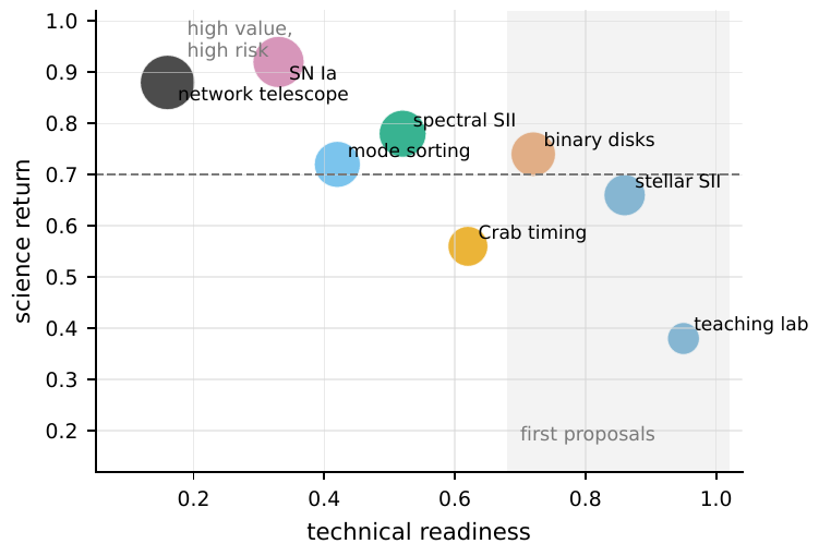
Figure 131 Technical maturity, scientific return, cost, and risk in a roadmap. Tasks in the upper-right region with high maturity are suitable for near-term proposals. Upper-left tasks have high scientific value but need pathfinder work first. Point size indicates cost pressure, while position gives the relative assessment of readiness and return.

The first 2026–2030 papers should be specific. An executable project might be “measure angular diameters for 10–30 bright stars near 416 nm with four IACTs, and release the correlator and calibration library.” Another might be “use one pipeline to compare \(|V|^2\) models for binaries, Be-star disks, and rapid rotators.” Each paper should release an event-table format description, a correlator version, a time-shift null test, a calibrator-star list, baseline geometry, and posterior samples. Then, even if some targets are not detected, the project leaves reusable instrument knowledge.

2030–2040: multichannel event tables

The medium-term goal is to extend “one blue filter and one \(|V|^2\) curve” into a multichannel event table. Spectrally resolved intensity interferometry can compare angular scales inside and outside emission lines. Polarization- resolved correlations can test magnetic geometry, scattering, and strong-field radiation. Picosecond event tables can turn photon statistics into a new time-domain data product. Spectral multiplexing is attractive because each spectral channel has a longer coherence time while many channels can add SNR in parallel. The cost is data rate, interchannel calibration, and a more complex dispersion model [Abe et al., 2024, Karl et al., 2022, Lai et al., 2021].

The basic data product for the multichannel phase can be written as

(363)\[\bm{d}= \left\{ H_{ab}^{\nu p}(\tau), \widehat{|V_{ab}^{\nu p}|^2}, C_{\nu_i\nu_j}^{p_i p_j}, \bm{\Sigma} \right\}.\]

\(H_{ab}^{\nu p}\) is the delay histogram for telescopes \(a,b\), frequency channel \(\nu\), and polarization channel \(p\). \(|V|^2\) is the calibrated spatial-coherence observable. \(C_{\nu_i\nu_j}^{p_i p_j}\) is a cross-frequency or cross-polarization covariance. \(\bm{\Sigma}\) is the covariance matrix of these data. Writing “multichannel quantum observation” is not enough; storage, normalization, and public release of these quantities determine whether the project has reached the engineering stage.

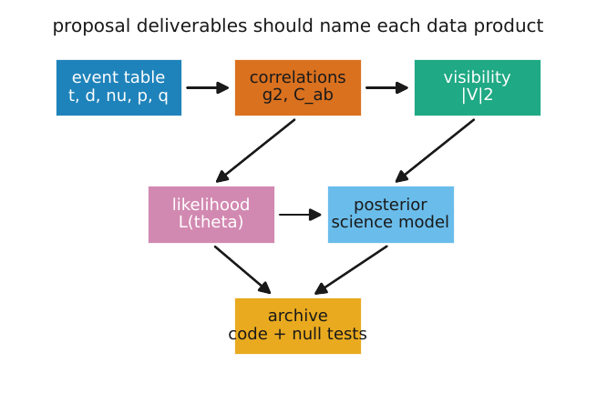
Figure 132 Product chain from proposal to public data. The event table preserves arrival time, telescope, frequency, polarization, and quality flags. The correlator turns it into g⁽²⁾ and covariance products. The spatial model produces |V|². The likelihood and posterior connect those quantities to astrophysical parameters. The archive must include code, versions, and null tests.

Type Ia supernova distances are a typical high-risk, high-return medium-term case. They require rapid triggering, kilometer to ten-kilometer baselines, explosion time, velocity model, photospheric asymmetry, and joint modeling of intensity-interferometry angular radii. The toy model by Kim, Nugent, Chen, and collaborators gives the feasibility boundary: only nearby, bright, early discoveries are worth interferometric follow-up [Kim et al., 2025]. Natural lasers, Crab pulsar photon statistics, Be-star disk lines, and AGN broad-line-region geometry can be written as the same class of plan, but each must first state trigger rate, observable window, background, and failure criteria.

After 2040: quantum-network telescopes

Long-term goals should be layered. Local mode sorting and phase-sensitive measurements do not require a full quantum network, and can already improve information efficiency for small separations and brightness moments [Tham et al., 2017, Tsang et al., 2016]. Two-photon astrometry, single-photon assistance, and linear-optics pathfinders aim to couple astronomical light stably to laboratory quantum resources [Marchese and Kok, 2023, Rajagopal et al., 2024]. Entanglement-assisted long-baseline interferometry requires entanglement distribution rate, quantum memory time, frequency-conversion efficiency, Bell fidelity, and astronomical synchronization to work together, so it belongs to a later stage [Modak and Kok, 2025, Padilla et al., 2026, Stas et al., 2026, Zhang and Jennewein, 2025].

The resource thresholds for quantum-network telescopes were written in Chapter Quantum network telescopes as constraints on link rate, storage time, and effective fidelity in Eqs. (334), (335), and (336). A proposal should put the same quantities into its acceptance table. \(R_{\rm ent}\) is the entangled-pair generation rate, in \({\rm s}^{-1}\). \(\eta_{\rm link}\), \(\eta_{\rm mem}\), and \(\eta_{\rm conv}\) are link, memory, and frequency-conversion efficiencies. \(R_{\gamma,{\rm useful}}\) is the astronomical photon rate that actually enters the target mode and time window. \(T_{\rm mem}\) is usable storage time. \(B/c\) is the baseline light-travel time. For \(B=1000\,{\rm km}\), \(B/c\simeq3.3\,{\rm ms}\). Ground-based kilometer baselines need only \(\mu{\rm s}\) to ms synchronization, but global or space baselines quickly increase the storage and distribution pressure. If link loss, memory decoherence, or useful photon rate misses the target, the network scheme is not yet ready to replace conventional intensity or amplitude interferometry.

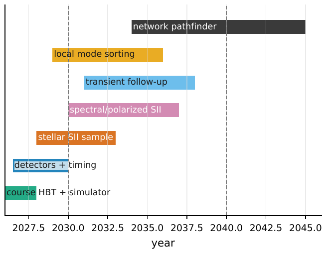
Figure 133 Staged timeline from course HBT to quantum-network pathfinders. Green and blue tasks build personnel, event tables, timing, and calibration. Orange and purple tasks produce first-generation science samples and multichannel correlations. The black long-term tasks should become facility roadmaps only after local mode sorting, links, and memory metrics have passed their gates.

How to write the research plan

An executable milestone names both the observable and the acceptance criterion:

(364)\[m_j= \left( O_j,\, \sigma_{O,j}^{\rm goal},\, T_j,\, N_{{\rm null},j},\, D_{{\rm release},j} \right).\]

\(O_j\) is the observable, such as \(g^{(2)}(0)-1\), \(|V|^2\), the angular scale ratio inside and outside a line, or \(D_A\). \(\sigma_O^{\rm goal}\) is the target precision. \(T_j\) is the due date or required observing time. \(N_{\rm null}\) is the number of null tests to be passed. \(D_{\rm release}\) is the data product to be released. A near-term project can require \(N_{\rm null}\ge2\), such as time shift and off source. A medium-term multichannel project should require \(N_{\rm null}\ge4\), such as time shift, off band, wrong polarization, and injection recovery. A long-term network project should also include independent gates on link fidelity and memory decoherence.

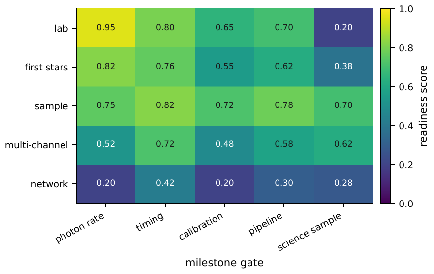
Figure 134 Milestone gate matrix for different phases. Course experiments and first-generation stellar SII are already relatively mature in photon rate, timing, and pipeline readiness, while multichannel calibration and the network phase still have large gaps. The numbers are examples of readiness scores that should be quantified in a proposal, not facility commitments.

The error budget should appear in the first proposal draft and should follow the decomposition in Eq. (344) of Chapter Observing design, error budgets, and feasibility calculations. \(\sigma_{\rm stat}\) comes from Poisson or correlation-count noise. \(\sigma_{\rm cal}\) comes from zero-baseline contrast, timing synchronization, polarization response, and spectral response. \(\sigma_{\rm bg}\) comes from night sky, continuum, or companion background. \(\sigma_{\rm model}\) comes from stellar-disk, supernova-photosphere, BLR, or maser geometry. \(\sigma_{\rm sel}\) comes from trigger, weather, and target selection. Statistical sampling can be implemented with MCMC, nested sampling, or posterior predictive checks, but these tools do not replace the physical error terms themselves [Cash, 1979, Feroz et al., 2009, Foreman-Mackey et al., 2013, Parsotan et al., 2025, Scargle et al., 2013].

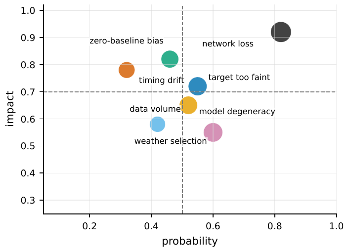
Figure 135 Risk register for the roadmap. Risks in the upper-right region need mitigation plans before the project begins. Network loss needs a short-baseline pathfinder, zero-baseline bias needs a calibrator library, and targets that are too faint need explicit trigger and abandonment criteria. Larger points indicate weaker mitigation.

The risk register should be written together with failure criteria. If the target is 1 mag fainter than expected, the photon rate falls to about 40%. If the systematic floor stalls at \(3\times10^{-5}\), many small \(|V|^2\) signals are no longer measurable. If a Type Ia trigger arrives 10 days late, the angular radius is larger but the luminosity has faded and model uncertainty has grown. If a network link delivers only a few high-fidelity entangled pairs per day, the science mode should fall back to local mode sorting or intensity interferometry. A roadmap may fail, but a useful failure says what must change in the next stage.

From course projects to research topics

Course projects can begin with Chapter Teaching experiments and computational experiments: tabletop HBT, event-table simulation, uniform-disk fitting, SPADE Fisher information, and false-alarm calculation. Smaller research topics work well when they center on one pipeline: timing synchronization, the correlator, a calibration library, target selection, or an open-data notebook. More complete science projects can target the line angular scale of Be-star H\(\alpha\) disks, multibaseline models of rapid rotators, phase-resolved photon statistics of the Crab pulsar, systematic errors in a Type Ia distance toy model, or a joint experiment combining local mode sorting with adaptive optics. Large collaborations can connect these topics to CTAO/IACT, ELT/VLTI/CHARA, Rubin, SKA, LIGO/Virgo/KAGRA/ET, or quantum-network laboratories.

A project should list at least the new observable, event-table fields, data estimation steps, symbol units, typical ranges, two or more null tests, and the data, code, or instrument constraint that remains useful if the main target fails. Such a plan can be reproduced, reviewed, and improved. Otherwise, “quantum” remains only in the title.