Why quantum astronomy is needed

Chapter opening

Conventional astronomy already has images, spectra, light curves, and polarimetry. Quantum astronomy does not replace those data products. It starts one step earlier, with the photon event table behind them, and keeps the joint probabilities among arrival time, receiver position, frequency, and polarization. Mean intensity tells us how much light arrived. Correlation functions and mode measurements tell us how the photons arrived together. This extra information has already been measured in HBT experiments, the Narrabri stellar intensity interferometer, stellar photon bunching, and modern VERITAS and MAGIC intensity interferometry. It is not the same thing as quantum gravity, and it is not just photon counting [Abeysekara et al., 2020, Abe et al., 2024, Guerin et al., 2017, Hanbury Brown, 1956, Hanbury Brown, 1974].

Conventional astronomy compresses the event table into mean quantities

Chapter Mathematical and Physical Foundations wrote a single photon event in the form of Eq. (1): arrival time, receiver position, frequency channel, polarization label, and weight form the minimal event row. The question now is what is lost when this table is compressed. An image, a spectrum, a light curve, and a conventional polarimetric measurement are different marginalizations of the same event table.

An image estimates the mean intensity on the sky. If the events are binned in angular coordinates \((x,y)\), with pixel solid angle \(\Delta\Omega\), exposure time \(\Delta t\), and frequency bandwidth \(\Delta\nu\), then

(43)\[\hat I(x,y)\simeq \frac{N(x,y)} {A_{\rm eff}\,\eta\,\Delta t\,\Delta\nu\,\Delta\Omega}.\]

Here \(N(x,y)\) is the weighted photon count in the pixel, \(A_{\rm eff}\) is the effective collecting area in \(\mathrm{m^2}\), \(\eta\) is the total throughput, and \(\Delta\Omega\) is measured in steradians. A spectrum bins the same table in \(\nu\). A light curve bins it in \(t\). A standard polarization measurement combines the mean intensities in several polarization channels into Stokes parameters. These are mostly first-order statistics.

First-order statistics do not keep track of which events came together. After \(10^8\) events have been compressed into a light curve, the total count in each time bin is still known, but the pair structure inside the bin has gone: which events were separated by a few picoseconds, which belonged to a given telescope pair, and which shared the same frequency-polarization mode. For many astrophysical questions that compression is exactly what one wants. For intensity interferometry, photon bunching, cross-line correlations, polarization-resolved correlations, and optimal parameter estimation, it removes the signal.

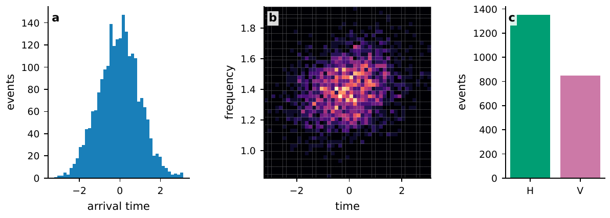
Figure 7 A photon event table stores arrival time, telescope position, frequency channel, and polarization label in one data structure. Marginalizing over a single coordinate gives a light curve, a spectrum, or a polarization intensity. Keeping event pairs gives delay histograms, intensity correlations, and cross-channel covariances.

In Fig. Figure 7, the left panel keeps only the marginal distribution of arrival times, the middle panel keeps a joint distribution in time and frequency, and the right panel keeps polarization channel counts. The observables of quantum astronomy usually begin with the middle panel, or with still higher-dimensional pair statistics, rather than with a single-channel curve that has already been averaged.

Equal mean intensity does not imply equal joint probability

Let \(a\) denote an event label. It may be a time bin, a telescope index, a frequency channel, or a polarization channel. The first-order probability \(P_1(a)\) gives the probability that one event falls in \(a\). The second-order probability \(P_2(a,b)\) gives the joint probability that two events fall in \(a\) and \(b\). If the events are independent,

(44)\[P_2(a,b)=P_1(a)P_1(b).\]

Everything that remains after subtracting this product is correlation information. In count language, the covariance between two channels \(a\) and \(b\) is

(45)\[C_{ab}=\langle N_aN_b\rangle-\langle N_a\rangle\langle N_b\rangle.\]

\(N_a\) and \(N_b\) are event counts in the same time window, or in windows separated by a specified lag. If \(C_{ab}=0\), the two channels have no measurable common fluctuation. If \(C_{ab}>0\), they have excess joint arrivals. If \(C_{ab}<0\), the first suspects are dead time, exclusion effects, selection functions, or genuine antibunching.

The normalized second-order correlation is

(46)\[g^{(2)}_{ab}(\tau)= \frac{\langle N_a(t)N_b(t+\tau)\rangle} {\langle N_a(t)\rangle\langle N_b(t+\tau)\rangle}.\]

The delay \(\tau\) is measured in seconds. This quantity can be estimated directly from an event table. One first builds a delay histogram of event pairs between channel \(a\) and channel \(b\), then divides by the accidental coincidence level implied by the two single-channel count rates. The baseline \(g^{(2)}=1\) corresponds to independent arrivals. Values above unity indicate bunching or a common fluctuation. Values below unity may indicate nonclassical antibunching, but in an astronomical detector they may also come from dead time, pile-up, or selection effects.

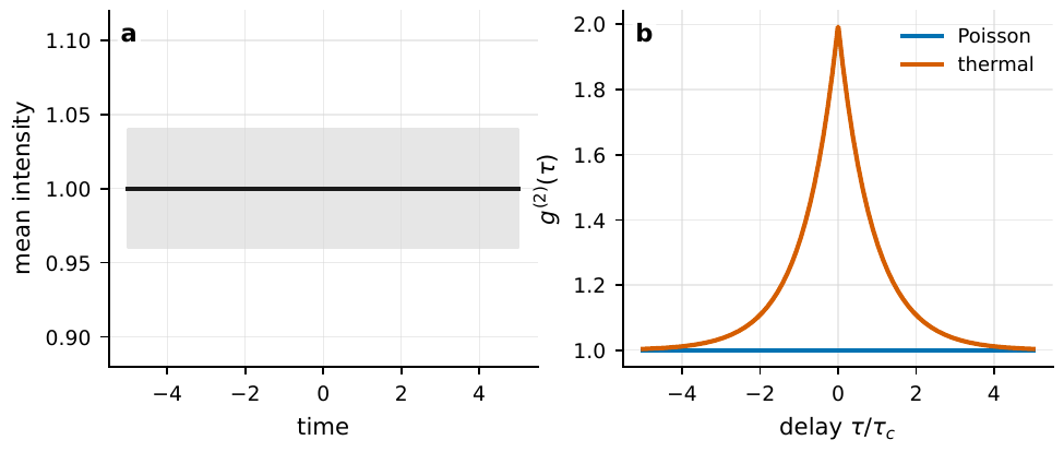
Figure 8 Two light beams can have the same mean intensity and different second-order correlations. Poisson light has g⁽²⁾ ≃ 1. Thermal light has an excess probability of joint arrivals within the coherence time, so g⁽²⁾(0) > 1.

Figure Figure 8 separates mean intensity from second-order statistics. The mean intensity is identical in the left panel. The thermal field has a short-delay correlation peak in the right panel. A standard light curve sees the left panel. An HBT measurement sees the right panel.

Thermal light, coherent light, and multimode dilution

Coherent and thermal light can be equally bright and still have different photon statistics. An ideal coherent state has an approximately Poisson count distribution,

(47)\[P_{\rm coh}(N)=e^{-\mu}\frac{\mu^N}{N!},\qquad g^{(2)}_{\rm coh}(0)=1.\]

The parameter \(\mu\) is the mean photon number in one time-frequency-polarization-space mode. A single-mode thermal field has

(48)\[P_{\rm th}(N)=\frac{\bar n^N}{(1+\bar n)^{N+1}},\qquad g^{(2)}_{\rm th}(0)=2.\]

\(\bar n\) is the mean occupation number of that mode. The value \(g^{(2)}(0)=2\) in Eq. (48) means that the zero-delay joint arrival probability is twice the value expected for an independent Poisson process. This is thermal photon bunching. It is also the experimental doorway through which the HBT effect entered quantum optics. Glauber’s coherence theory and the review by Mandel and Wolf recast the same physics in the language of field correlation functions [Glauber, 1963, Mandel and Wolf, 1965, Mandel and Wolf, 1995].

Real astronomical observations are almost never single-mode measurements. If the instrument collects \(M\) mutually incoherent modes, the thermal bunching contrast is approximately

(49)\[g^{(2)}(0)-1\simeq \frac{1}{M}.\]

The effective mode number includes time, frequency, spatial, and polarization modes. A broad optical filter increases the number of frequency modes. A large field of view or a multimode fiber increases the number of spatial modes. Unresolved polarization mixes two polarization modes. The classic experiment of Martienssen and Spiller already showed how coherence and intensity fluctuations are tied together, and later measurements of solar and blackbody photon bunching used narrow filtering and mode control to make the signal observable [Martienssen and Spiller, 1964, Tan et al., 2014].

Finite timing resolution dilutes the peak again. The coherence time is roughly

(50)\[\tau_c\simeq \frac{1}{\Delta\nu},\]

where \(\Delta\nu\) is the optical bandwidth in Hz. If the electronic time bin or detector response width satisfies \(\Delta t\gg\tau_c\), the observed contrast is roughly

(51)\[g^{(2)}_{\rm obs}(0)-1 \simeq \frac{1}{P\,M}\frac{\tau_c}{\Delta t}.\]

Here \(P\) is the polarization dilution factor. Selecting one polarization gives \(P\simeq1\); unresolved random polarization often gives a dilution close to 2. \(M\) is the effective mode number, and \(\Delta t\) is the detector response or the analysis bin. Equation (51) is an order-of-magnitude relation. A real analysis must convolve the filter transmission, detector jitter, electronic bandwidth, and correlator response. Tan et al. note in the full blackbody photon-bunching analysis that the intrinsic coherence time of optical blackbody light can be as short as \(10^{-14}\,\mathrm{s}\), whereas common single-photon detectors respond on tens of picoseconds. Narrowband filtering is therefore usually needed to stretch \(\tau_c\) into an accessible range [Tan et al., 2014].

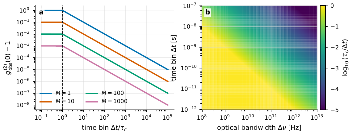
Figure 9 Second-order correlation contrast is reduced by both effective mode number and finite timing resolution. The left panel shows how \(g^{(2)}_{\rm obs}(0)-1\) falls as the mode number M grows, or as the time bin Δt becomes longer than the coherence time τ_c. The right panel substitutes τ_c ≃ 1/Δν and shows why broad optical bandwidths and slow electronics make the bunching peak small.

Figure Figure 9 gives the scale in a real telescope. For \(\Delta\nu=10^{12}\,\mathrm{Hz}\), the coherence time is \(\tau_c\sim1\,\mathrm{ps}\). With a \(1\,\mathrm{ns}\) electronic response, even a single-mode, single-polarization thermal signal is reduced to a contrast of order \(10^{-3}\). Multimode collection, background light, and polarization dilution can push astronomical signals down to \(10^{-6}\)–\(10^{-3}\).

From HBT to Narrabri

Hanbury Brown and Twiss proposed measuring spatial coherence through correlated intensity fluctuations, instead of coherently combining the optical fields from two telescopes. For chaotic thermal light, the Siegert relation gives

(52)\[g^{(2)}_{12}(0)-1=|\gamma^{(1)}_{12}|^2\]

in the ideal limit of a single mode, one polarization, and infinitely fast detectors. \(\gamma^{(1)}_{12}\) is the first-order coherence between the two telescopes. In an actual observation, the right-hand side is multiplied by the timing, mode, and polarization dilution factors discussed around Eq. (51).

The spatial coherence is linked to the Fourier transform of the sky brightness. For a uniform disk of angular diameter \(\theta\),

(53)\[|\gamma^{(1)}(B)|^2 = \left[ \frac{2J_1(\pi B\theta/\lambda)} {\pi B\theta/\lambda} \right]^2.\]

\(B\) is the projected baseline, \(\lambda\) is the wavelength, and \(J_1\) is the first-order Bessel function. Longer baselines resolve the disk more strongly and drive \(|\gamma^{(1)}|^2\) downward. Intensity interferometry does not measure the complex phase, but it does measure this squared visibility curve. That is enough to fit stellar angular diameters, limb darkening, and binary models.

The Sirius test and the Narrabri stellar intensity interferometer turned this idea into astronomy. Narrabri used two 6.5 m light collectors to measure angular diameters of hot stars. The final program produced angular diameters for 32 stars, and related papers worked out how limb darkening changes the conversion from a uniform-disk diameter to a physical stellar diameter [Hanbury Brown, 1956, Hanbury Brown, 1974, Hanbury Brown et al., 1967, Hanbury Brown et al., 1974, Hanbury Brown et al., 1967, Hanbury Brown et al., 1974].

The influence of HBT extends beyond astronomy. Baym’s review follows the same two-particle correlation idea from stars to nuclear collisions. In both cases, the width of a correlation function is related to the size of the emitting region. The details differ. Heavy-ion interferometry must handle final-state interactions, Coulomb corrections, and nonchaotic components. Astronomical photon measurements must handle detector response, background, mode number, and bandwidth [Baym, 1998, Boal et al., 1990]. HBT is therefore not just an instrumental trick. It is a way of inferring source structure from second-order joint probabilities.

Why the field faded, and why it came back

Intensity interferometry went quiet for decades mainly because the signal was small, not because the physics was wrong. If the source has spectral photon flux density \(n\), in \(\mathrm{photons\,s^{-1}\,m^{-2}\,Hz^{-1}}\), the classical signal-to-noise ratio for one telescope pair scales as

(54)\[{\rm SNR}\simeq A\,\alpha\,n\,|\gamma^{(1)}_{12}|^2 \sqrt{\frac{\Delta f\,T}{2}}.\]

\(A\) is the geometric mean of the two collecting areas in \(\mathrm{m^2}\), \(\alpha\) is the total quantum efficiency, \(\Delta f\) is the electronic bandwidth in Hz, and \(T\) is the integration time. This scaling explains why progress after Narrabri was hard. The direct resources are collecting area, quantum efficiency, electronic bandwidth, and time on target. Dravins et al. emphasized in the CTA studies that intensity interferometry relaxes optical path tolerances to electronic time scales: a nanosecond response corresponds to centimeter-to-meter path tolerances. The price is severe dilution, because the optical coherence time is much shorter than the electronic response [Dravins et al., 2012, Dravins et al., 2013].

The modern revival is mostly an engineering story. Large Cherenkov telescope arrays provide huge collecting areas that already exist. Photomultipliers, APDs, SPADs, and fast electronics can record fluctuations on nanosecond and sometimes picosecond scales. FPGA, GPU, and offline correlators can duplicate data streams across many baseline pairs. Precise timing and digital delay correction can track geometric path differences without stabilizing the optical phase to nanometers. The engineering roadmaps in the Le Bohec–Holder work, the Dravins CTA papers, and later CTA layout simulations are consistent: the signal is weak, but an electronic correlator can be replicated; rough optical paths still work; and a multi-telescope array turns \(u,v\) coverage into the main asset [Dravins et al., 2012, Dravins et al., 2013, Jensen et al., 2010, Le Bohec et al., 2008, Le Bohec and Holder, 2006, Nuñez et al., 2010].

Recent measurements have moved beyond proof of concept. Guerin et al. measured temporal photon bunching from Arcturus, Procyon, and Pollux with 1 m telescopes in photon-counting mode. The peak contrast was about \(2\times10^{-3}\), and the noise followed the expected shot-noise scaling [Guerin et al., 2017]. The VERITAS intensity-interferometry system, using four 12 m Cherenkov telescopes, measured sub-milliarcsecond angular diameters of \(\beta\) CMa and \(\epsilon\) Ori with better than 5 percent precision, and showed that multibaseline offline correlation scales in practice [Abeysekara et al., 2020]. The two 17 m MAGIC Cherenkov telescopes have also performed optical intensity interferometry, with later system papers reporting performance and first measurements [Abe et al., 2024, Acciari et al., 2020]. The Aqueye/Iqueye Vega photon-counting experiment showed a different side of the same problem: high-time-resolution event tables, zero-baseline correlations, and the systematic errors that appear when kilometer-scale baselines must be calibrated [Zampieri et al., 2021].

These experiments make the boundary of first-generation projects concrete. If an event table preserves time, position, frequency, and polarization labels, some second-order observables can already be measured. The hard parts are weak signals, many systematics, and bright target requirements. The concept itself is not speculative.

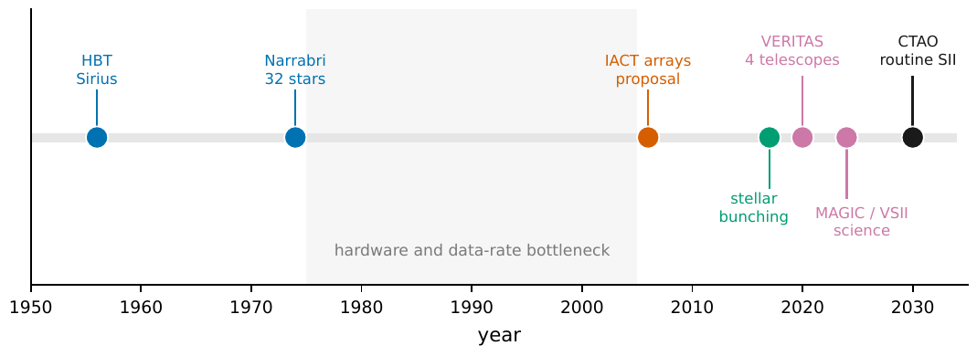
Figure 10 Timeline of optical intensity interferometry from HBT and Narrabri to the revival with Cherenkov telescope arrays. The quiet period after the 1970s mainly reflected engineering limits in collecting area, fast detection, and multibaseline correlation. IACT arrays, digital correlators, and photon-counting event tables have gradually removed those limits.

A working definition: what counts as quantum astronomy

In this book, quantum astronomy means event-level astronomy of astrophysical light fields: the study of joint probabilities, coherence functions, and mode information, used to answer questions about sources, propagation, fundamental physics, or observing strategy. Its basic data object is a labelled photon event table, not only a mean-intensity data product. Instruments such as Iqueye and Aqueye were designed with exactly this premise: astronomical photons should be treated as time-tagged events with nanosecond or better precision [Capraro et al., 2010].

The common observables are correlation functions, joint probabilities, and mode projections. A compact notation is

(55)\[G^{(n)}(1,\ldots,n)= \left\langle \hat E_1^{(-)}\cdots \hat E_n^{(-)} \hat E_n^{(+)}\cdots \hat E_1^{(+)} \right\rangle,\]

where each index may include time, position, frequency, and polarization. \(n=1\) gives ordinary mean intensity. \(n=2\) gives HBT correlations and photon bunching. \(n=3\) can help recover partial phase information in multi-telescope intensity interferometry. Equation (55) is not abstract notation floating above the data. It corresponds to single, double, or multiple coincidence statistics in an event table.

This boundary is deliberately practical. Quantum astronomy is not quantum gravity, and it is not every cosmological argument that uses the word “quantum”. If a question cannot be written as an estimable event-table observable with an error model and a null test, it is not yet an observing program. Conversely, photon counting alone is not automatically quantum astronomy. It enters the scope of this book when the joint statistics, mode structure, or optimal measurement of individual events carries information that mean intensity does not.

First-generation science cases

The safest starting point is bright stars. Intensity interferometry can measure angular diameters, limb darkening, rotational flattening, binary separations, and hot-star wind structure. Such stars are bright, close to thermal light sources, and often have angular scales from \(0.05\) to a few milliarcseconds. That range lies naturally on visible-light baselines of hundreds of meters to kilometers. The Narrabri results, the modern VERITAS and MAGIC diameter measurements, the \(\beta\) UMa angular diameter, and the \(\gamma\) Cas flattening measurement all put bright stars at the front of the first-generation target list [Abeysekara et al., 2020, Abe et al., 2024, Acharyya et al., 2024, Archer et al., 2025, Hanbury Brown et al., 1974].

Sources with strong time structure offer a second route. Pulsars, bursts, novae, supernovae, and microlensing events put arrival time at the centre of the measurement. If two unresolved optical paths differ by a small delay, the delay structure of photon bunching may carry additional information. Saha proposed using photon bunching to measure microlens masses, and Lewis and Tuthill later examined decoherence in that idea. The physical point is that coherence time, source size, and propagation path difference must be treated together [Lewis and Tuthill, 2020, Saha, 2019].

Frequency- and polarization-resolved correlations push the method toward radiation physics. \(g^{(2)}(\tau)\) inside and outside a spectral line can be connected to coherence time and line width. Polarization-resolved correlations can test emission mechanisms, magnetic geometry, and propagation effects. Photon-correlation spectroscopy of natural lasers, blackbody photon bunching, and X-ray driven photon bunching all show that the HBT idea is not limited to stellar angular diameters. It can also diagnose line widths, excitation processes, and high-energy variability [Dravins and Germanà, 2008, Johansson and Letokhov, 2005, Katznelson et al., 2024, Tan et al., 2014]. These directions are farther from routine survey astronomy, but the chain of reasoning is the same: start with the event table, measure photon statistics, and connect those statistics to radiation, propagation, and fundamental physics.

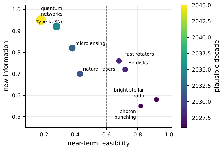
Figure 11 Feasibility and added information for first-generation quantum astronomy science cases. Bright-star angular diameters and stellar photon bunching are already close to routine observation. Be-star disks, rapidly rotating stars, and natural lasers are near-term extensions. Type Ia supernova angular distances and quantum-network telescope science have high value, but require longer baselines, rapid triggering, or quantum-link engineering.

Observable	Typical range	Main limitation
\(R_\gamma\)	\(10^5\) to \(10^9\,\mathrm{s^{-1}}\) can be reached for bright stars in one channel	Detector saturation, dead time, background, and data rate.
\(\Delta t\)	\(10\,\mathrm{ps}\) to \(10\,\mathrm{ns}\)	Detector jitter, electronic bandwidth, mirror isochronicity, and clock synchronization.
\(\Delta\nu\)	\(10^9\) to \(10^{13}\,\mathrm{Hz}\)	Narrow bands increase coherence time but reduce photon rate; broad bands do the opposite.
\(g^{(2)}-1\)	\(10^{-6}\) to \(10^{-3}\) is common in astronomical intensity interferometry	Mode number, timing dilution, polarization dilution, and background dilution.
\(B\)	\(10\,\mathrm{m}\) to \(10\,\mathrm{km}\)	Sets the angular scale; long baselines have weaker signals and need more photons and better models.
$	\gamma^{(1)}	^2$

Exercises

Exercise 1. A thermal source is observed through a narrow filter with \(\Delta\nu=2\times10^{10}\,\mathrm{Hz}\). The detector response time is \(\Delta t=500\,\mathrm{ps}\). Assume one selected polarization and effective mode number \(M=1\). Use Eq. (51) to estimate \(g^{(2)}_{\rm obs}(0)-1\).

Exercise 2. Two telescopes observe the same uniform-disk star at \(\lambda=420\,\mathrm{nm}\), with \(\theta=0.6\,\mathrm{mas}\). Use Eq. (53) to calculate \(|\gamma^{(1)}|^2\) at \(B=50\,\mathrm{m}\), \(100\,\mathrm{m}\), and \(150\,\mathrm{m}\).

Exercise 3. Decide whether each observation belongs to the working definition of quantum astronomy used in this book, and explain why: ordinary CCD imaging; nanosecond photon time-stamp statistics of a pulsar; a broadband light curve that records only total flux; intensity correlations between two telescopes; polarization-resolved \(g^{(2)}_{HV}\).