Propagation effects: plasma, dust, and gravitational lensing

Chapter opening

On the way from source to telescope, photons pass through free electrons, turbulent magnetized plasma, dust grains, Earth’s atmosphere, and curved spacetime. Propagation changes arrival time, frequency, polarization, direction, and count correlations in the event table. Cold plasma produces \(\nu^{-2}\) dispersion and Faraday rotation. Turbulence produces scattering tails and scintillation. Dust produces extinction, reddening, and polarization selection. Gravitational lensing duplicates paths and creates magnification and time delay. The NE2001 and YMW16 electron-density models, the baryon census from localized FRBs, reviews of interstellar scattering, dust-extinction laws, and time-delay cosmography all set the relevant scales [Bhat et al., 2004, Cardelli et al., 1989, Cordes and Lazio, 2002, Fitzpatrick, 1999, Macquart et al., 2020, Refsdal, 1964, Refsdal, 1964, Rickett, 1977, Rickett, 1990, Treu and Marshall, 2016, Yao et al., 2017].

Propagation as a channel with memory

The telescope records the field after propagation. If two polarizations, many frequency channels, and several spatial modes are collected into one vector, propagation can be written as

(260)\[{\bf a}_{\rm out}(\omega,\hat{\bf n}) = {\bf S}(\omega,\hat{\bf n})\,{\bf a}_{\rm src}(\omega,\hat{\bf n}) +{\bf n}_{\rm fg}(\omega,\hat{\bf n}) ,\]

where \({\bf a}_{\rm src}\) is the annihilation operator or classical field-mode amplitude emitted by the source, \({\bf S}\) is the propagation matrix, and \({\bf n}_{\rm fg}\) represents foreground thermal radiation, sky background, and detector-chain noise. If the medium only absorbs and does not scatter, \({\bf S}\) is nearly diagonal. Faraday rotation mixes the two linear polarizations. Scattering and lensing mix both direction and arrival time. In the time domain, the same statement is

(261)\[E_{{\rm out},i}(t) = \sum_j\int h_{ij}(t-t')\,E_{{\rm src},j}(t')\,{\rm d}t' + n_i(t) ,\]

where \(i,j\) label polarization, telescope, image, or frequency channel. The units of \(h_{ij}\) depend on how the electric field is normalized. In pulse and intensity-correlation analysis, the most useful properties are its temporal width, peak delay, and relative phase between channels. Barycentric correction, clock offsets, atmospheric delay, and instrumental electronic delay also belong to this response. Pulsar timing models separate such terms down to the nanosecond level, making them one of the most mature calibrations in high-time-resolution astronomy [Edwards et al., 2006].

An event-table photon candidate can be written as \((t_q,\nu_q,p_q,{\bf x}_q,w_q)\). Here \(t_q\) is arrival time in seconds, \(\nu_q\) is frequency in Hz, \(p_q\) is polarization channel, \({\bf x}_q\) is pixel, baseline, or telescope index, and \(w_q\) is a quality weight. The propagation model maps source-side labels into observed labels. Dispersion mainly changes \(t_q(\nu_q)\). Faraday rotation changes \(p_q(\lambda_q^2)\). Scattering turns a narrow pulse into a broadened arrival time distribution with a long tail. Dust changes the acceptance probability as a function of \(\lambda_q\). Lensing copies one source event into several \({\bf x}_q\) values and several \(t_q\) values.

Propagation error budgets are often set by a few large scales. High-latitude Galactic DM is commonly \(30\)–\(100\,{\rm pc\,cm^{-3}}\); FRBs can reach \(10^3\)–\(10^4\,{\rm pc\,cm^{-3}}\). DM is measured from the slope of pulse arrival time with \(\nu^{-2}\). Ordinary interstellar RMs are often \(1\)–\(10^2\,{\rm rad\,m^{-2}}\), while dense magnetized environments can reach \(10^4\)–\(10^5\,{\rm rad\,m^{-2}}\). RM is measured from the slope of linear-polarization angle with \(\lambda^2\). Scattering broadening \(\tau_{\rm sc}\) can range from \(\mu{\rm s}\) to seconds and grows rapidly at low frequency; at fixed DM, it can differ by orders of magnitude between lines of sight. Optical extinction is often below \(0.1\) mag at high Galactic latitude, but several magnitudes in the Galactic plane and molecular clouds. Lensing delays span an even wider range: planetary or stellar lenses can give \(\mu{\rm s}\)–ms delays, while galaxy-scale strong lenses usually give days to years.

Cold plasma: dispersion, RM, and magnetic fields

For \(\omega\gg\omega_p\), the refractive index of a cold plasma is

(262)\[n(\omega)\simeq 1-\frac{\omega_p^2}{2\omega^2}, \qquad \omega_p^2=\frac{4\pi n_e e^2}{m_e}.\]

\(n_e\) is the free-electron number density in \({\rm cm^{-3}}\). The warm ionized medium of the Milky Way is often \(10^{-2}\)–\(10^{-1}\,{\rm cm^{-3}}\), while HII regions and local FRB environments can be much denser. Integrating the group delay gives the dispersion measure,

(263)\[{\rm DM}=\int n_e\,{\rm d}l ,\]

where \({\rm d}l\) is in pc, so DM has units \({\rm pc\,cm^{-3}}\). The cold-plasma delay between two radio channels is

(264)\[\Delta t_{\rm DM} = 4.148808\,{\rm ms}\, {\rm DM} \left[ \left(\frac{\nu_1}{\rm GHz}\right)^{-2} - \left(\frac{\nu_2}{\rm GHz}\right)^{-2} \right].\]

For \({\rm DM}=300\,{\rm pc\,cm^{-3}}\), the delay of \(0.6\) GHz relative to \(1.4\) GHz is about \(2.9\) s; between \(1.2\) and \(1.5\) GHz the same event differs by only about \(0.36\) s. Searches for radio pulses and FRBs usually dedisperse over a grid of trial DMs and then search for the peak signal-to-noise. Finite channel width \(\Delta\nu\) also causes intra-channel smearing,

(265)\[\Delta t_{\rm chan} \simeq 8.3\,\mu{\rm s}\, \left(\frac{{\rm DM}}{{\rm pc\,cm^{-3}}}\right) \left(\frac{\Delta\nu}{\rm MHz}\right) \left(\frac{\nu}{\rm GHz}\right)^{-3}.\]

The left side can be estimated from the pulse width in each channel of a dynamic spectrum. The right side shows that high DM, wide channels, and low frequencies directly wash out microsecond structure.

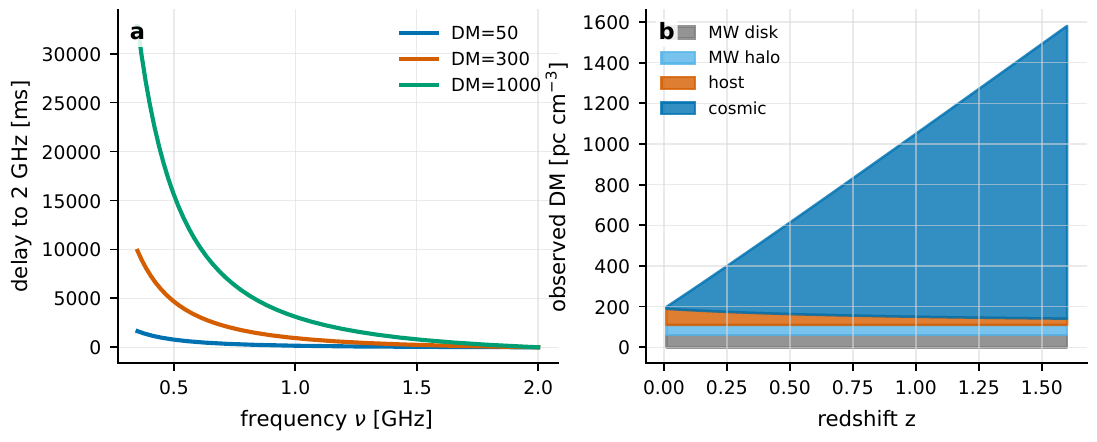
Figure 78 Cold-plasma dispersion and the FRB DM budget. The left panel shows arrival-time delay as a function of frequency, referenced to \(2\,{\rm GHz}\). The steep ν⁻² behavior at low frequency makes DM easy to estimate from a broadband dynamic spectrum. The right panel decomposes the observed DM of a localized FRB into the Milky Way disk, Galactic halo, host galaxy, and cosmological plasma. The host term enters the observed value with a (1 + z)⁻¹ factor because both frequency and time interval are redshifted; the cosmological term grows approximately with redshift at z ≲ 1.

The Milky Way electron density is far from constant. NE2001 combines a thick disk, thin disk, spiral arms, local cavities, and clumps, with pulsar DMs, independent distances, and scattering data used as constraints. YMW16 updated the thick disk, thin disk, spiral arms, Galactic center, and treatments of the Magellanic Clouds and IGM; it is used to convert pulsar or FRB Galactic DM into distance or foreground estimates [Cordes and Lazio, 2002, Yao et al., 2017]. At high Galactic latitude, the disk contribution is often \(30\)–\(100\,{\rm pc\,cm^{-3}}\), and the halo contribution is commonly taken to be \(50\)–\(100\,{\rm pc\,cm^{-3}}\) in order of magnitude. Near the Galactic plane, HII regions, or supernova remnants, local structure can dominate over the smooth model.

For cosmological FRBs, one often writes

(266)\[{\rm DM}_{\rm FRB} = {\rm DM}_{\rm MW,ISM} +{\rm DM}_{\rm MW,halo} +{\rm DM}_{\rm cosmic}(z) +\frac{{\rm DM}_{\rm host}}{{1+z}} .\]

The host-galaxy term is divided by \(1+z\), because the observed frequency and time interval have both been stretched by redshift. In a homogeneous-universe approximation,

(267)\[{\rm DM}_{\rm cosmic}(z) = \frac{3cH_0\Omega_b f_{\rm IGM}}{8\pi Gm_p} \int_0^z \frac{f_e(z')(1+z')}{\sqrt{\Omega_m(1+z')^3+\Omega_\Lambda}} {\rm d}z' ,\]

where \(\Omega_b\) is the baryon density parameter, \(f_{\rm IGM}\) is the fraction of baryons in the diffuse IGM, and \(f_e\) is the number of free electrons per baryon. Localized FRB samples now measure the \({\rm DM}_{\rm cosmic}\)-\(z\) relation well enough to infer the cosmic baryon content. The scatter comes from cosmic-web inhomogeneity and is often written in a form such as \(\sigma_{\rm DM}\simeq F z^{-1/2}\), with \(F\sim0.1\)–0.4 representing different baryon-feedback and halo-gas distributions [Macquart et al., 2020, Spitler et al., 2014].

In magnetized plasma, the two circular polarizations have different phase velocities, so the linear-polarization angle rotates with wavelength squared:

(268)\[\psi(\lambda)=\psi_0+{\rm RM}\,\lambda^2 ,\]

(269)\[{\rm RM} = 0.812 \int \left(\frac{n_e}{{\rm cm^{-3}}}\right) \left(\frac{B_\parallel}{\mu{\rm G}}\right) \left(\frac{{\rm d}l}{\rm pc}\right) {\rm rad\,m^{-2}} .\]

\(B_\parallel\) is the magnetic-field component toward the observer. If DM and RM mostly arise in the same region, the line-of-sight mean magnetic field can be estimated as

(270)\[\langle B_\parallel\rangle \simeq 1.232\,\mu{\rm G}\, \frac{{\rm RM}/{\rm rad\,m^{-2}}}{{\rm DM}/{\rm pc\,cm^{-3}}}.\]

This is not a universal magnetic-field measurement. If RM comes from a magnetized host galaxy while most of DM comes from the IGM, Eq. (270) underestimates the local field. If the line of sight contains magnetic-field reversals, RM cancels while DM does not. RM studies of galaxy clusters and intergalactic gas usually handle these degeneracies together with X-ray gas density, radio halos, and grids of background sources [Carilli and Taylor, 2002].

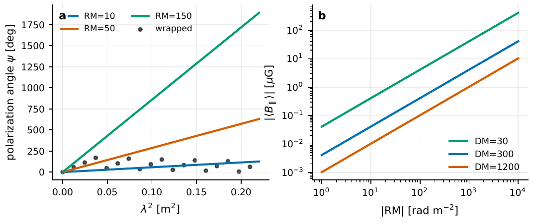
Figure 79 Two readings of Faraday rotation. The left panel shows the linear relation \(\psi=\psi_0+{\rm RM}\lambda^2\). Black points show that a real polarization angle is measured only modulo π, so narrow-band data can have wrapping ambiguities. The right panel plots \(\langle B_\parallel\rangle=1.232\,{\rm RM}/{\rm DM}\) as a function of RM; the same RM implies a stronger mean field in a lower-DM medium.

Scattering, scintillation, and dust

The interstellar electron density is not smooth. Small-scale turbulent fluctuations wrinkle the wavefront, producing angular broadening, pulse broadening, and intensity scintillation. In a single thin-screen approximation, the observed pulse is often written as a convolution,

(271)\[I_{\rm obs}(t) = \int I_{\rm src}(t')\,P(t-t')\,{\rm d}t', \qquad P(t)=\frac{1}{\tau_{\rm sc}}\exp\!\left(-\frac{t}{\tau_{\rm sc}}\right)H(t),\]

where \(P(t)\) is a one-sided exponential scattering kernel and \(H(t)\) is the Heaviside function. Real lines of sight may include multiple screens, anisotropic scattering, and finite source size, so the exponential tail is only the most common low-order model. The scattering time is often described by

(272)\[\tau_{\rm sc}\propto \nu^{-\alpha},\]

with \(\alpha\simeq4.4\) for a Kolmogorov thin screen. Multi-frequency pulsar samples give an empirical mean closer to \(\alpha=3.9\pm0.2\), with more than an order of magnitude of scatter at fixed DM [Armstrong et al., 1995, Bhat et al., 2004, Rickett, 1977, Rickett, 1990]. A commonly used empirical relation is

(273)\[\log_{10}\!\left(\frac{\tau_{\rm sc}}{{\rm ms}}\right) = -6.46 +0.154\log_{10}{\rm DM} +1.07(\log_{10}{\rm DM})^2 -3.86\log_{10}\!\left(\frac{\nu}{\rm GHz}\right),\]

where DM is in \({\rm pc\,cm^{-3}}\). This formula is useful for scale estimates, not as a substitute for measuring scattering along each line of sight. For \({\rm DM}=300\,{\rm pc\,cm^{-3}}\), it gives roughly millisecond broadening at \(1.4\,{\rm GHz}\); at \(600\,{\rm MHz}\), broadening can increase to more than ten milliseconds. In a dynamic spectrum, the decorrelation bandwidth \(\Delta\nu_d\) and pulse broadening are approximately related by

(274)\[\tau_{\rm sc}\simeq \frac{C_1}{2\pi\Delta\nu_d},\]

where \(C_1\) depends on geometry and the scattering spectrum and is usually of order unity. In strong scattering, \(\Delta\nu_d\) is narrow and broadband averaging erases scintillation. In weak scattering, the scintillation pattern drifts with time and frequency and can instead measure screen velocity, screen distance, and source angular size.

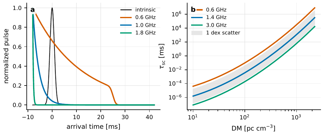
Figure 80 Interstellar scattering turns a short pulse into an arrival-time distribution with a long tail. The left panel convolves a narrow Gaussian pulse with a one-sided exponential kernel; lower frequencies have longer tails because \(\tau_{\rm sc}\propto\nu^{-4}\). The right panel uses the empirical relation to show how \(\tau_{\rm sc}\) varies with DM and frequency. The gray band marks the order-of-magnitude scatter commonly seen at fixed DM.

Plasma can also refract like a lens. Transverse gradients in electron column density create a frequency-dependent phase screen, bend lower-frequency rays more strongly, and can produce caustics, multiple imaging, and narrow-band magnification. Gaussian plasma lenses, plasma structures in FRB host galaxies, and gravitational-lensing corrections in inhomogeneous plasma all show that, after removing the \(\nu^{-2}\) dispersion law, residual structure may still be propagation-driven [Bisnovatyi-Kogan and Tsupko, 2010, Clegg et al., 1998, Cordes et al., 2017, Er and Mao, 2014]. Toward the Galactic center, millimeter VLBI must also handle a strong scattering screen. Event-horizon-scale imaging of Sgr A* has to model intrinsic source structure, scattering blur, and time variability together [Doeleman et al., 2008, Event Horizon Telescope Collaboration et al., 2022, Event Horizon Telescope Collaboration et al., 2022].

For optical and infrared photons, dust behaves like a loss channel with wavelength and polarization selection. The flux relation is

(275)\[F_{\lambda,{\rm obs}} = F_{\lambda,{\rm int}}\,10^{-0.4A_\lambda},\]

where \(A_\lambda\) is in magnitudes. Selective extinction is written

(276)\[E(B-V)=A_B-A_V, \qquad R_V=\frac{A_V}{E(B-V)}.\]

The Milky Way average is \(R_V\simeq3.1\). Diffuse interstellar lines of sight are often near \(2.5\)–3.5, while dense clouds can exceed \(5\), meaning that larger grains make extinction grayer. The Cardelli–Clayton–Mathis law writes the infrared, optical, and ultraviolet average curve as a one-parameter family in \(R_V\). Fitzpatrick showed that real lines of sight still have substantial scatter, especially in the strength of the \(2175\,\text{\AA}\) bump and the far-UV rise [Cardelli et al., 1989, Draine, 2003, Fitzpatrick, 1999]. For a blue source with \(E(B-V)=0.2\) mag, correcting with an average extinction law can easily leave ultraviolet errors of \(0.1\) mag. For polarization angle, color temperature, and early transient SEDs, that is already a major systematic.

Non-spherical dust grains partially aligned with the magnetic field linearly polarize transmitted starlight. The common Serkowski relation is

(277)\[\frac{P(\lambda)}{P_{\max}} = \exp\!\left[-K\ln^2\!\left(\frac{\lambda_{\max}}{\lambda}\right)\right],\]

where \(\lambda_{\max}\) is usually near \(0.55\,\mu{\rm m}\), and the empirical upper envelope is about \(P_{\max}\simeq9E(B-V)\%\). Not every line of sight reaches this envelope. Grain shape, alignment efficiency, changes in magnetic field direction, and multiple dust layers all matter [Andersson et al., 2015, Serkowski et al., 1975]. Dust scattering can also turn a brief burst into a light echo or X-ray halo. If a dust screen lies at fraction \(x\) of the source-observer distance and the scattering angle is \(\theta\), the geometric delay is approximately

(278)\[\Delta t_{\rm dust} \simeq \frac{D_s}{2c}\frac{x}{1-x}\theta^2 ,\]

where \(D_s\) is source distance. For Galactic sources, arcsecond-scale scattering can give hour-to-day delays. For extragalactic sources, dust geometry and angular resolution have to enter the model together.

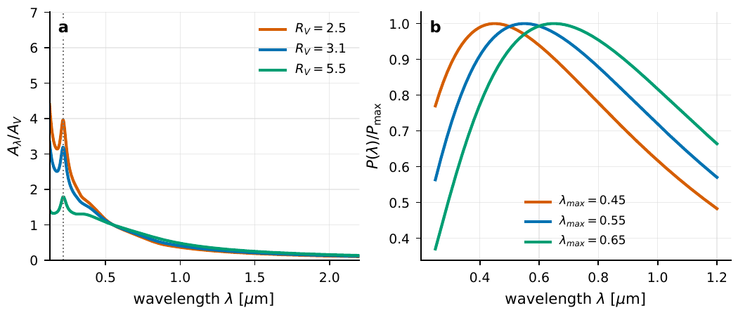
Figure 81 Dust changes photon color, flux, and polarization. The left panel shows the CCM mean extinction curve. Larger R_V makes optical and near-infrared extinction grayer; the ultraviolet bump near \(0.2175\,\mu{\rm m}\) diagnoses small grains and carbonaceous material. The right panel shows a Serkowski polarization curve, where shifts in λ_max reflect changes in grain size and alignment environment.

Gravitational lensing: multipath, time delay, and wave effects

Gravitational lensing does not change the photon’s frequency-dispersion relation, but it changes path, direction, and arrival time. In the thin-lens approximation,

(279)\[{\boldsymbol\beta} = {\boldsymbol\theta} - {\boldsymbol\alpha}({\boldsymbol\theta}),\]

where \({\boldsymbol\beta}\) is the true source position, \({\boldsymbol\theta}\) is the image position, and \({\boldsymbol\alpha}\) is the reduced deflection angle. All are usually measured in radians or arcseconds. For a point-mass lens, the Einstein angle is

(280)\[\theta_E = \left( \frac{4GM}{c^2} \frac{D_{ls}}{D_lD_s} \right)^{1/2}.\]

\(D_l\), \(D_s\), and \(D_{ls}\) are angular-diameter distances. A \(1\,M_\odot\) lens in Galactic-scale geometry gives a milliarcsecond \(\theta_E\). A galaxy-mass lens gives arcsecond-scale multiple-image separation. The magnification is

(281)\[\mu = \frac{1}{\det(\partial{\boldsymbol\beta}/\partial{\boldsymbol\theta})},\]

and \(|\mu|\) can be large near a caustic. Finite source size, microlensing, dust, and time sampling limit the actual observable peak.

Arrival time is controlled by the Fermat potential:

(282)\[t({\boldsymbol\theta},{\boldsymbol\beta}) = \frac{D_{\Delta t}}{c} \left[ \frac{1}{2}|{\boldsymbol\theta}-{\boldsymbol\beta}|^2 - \psi({\boldsymbol\theta}) \right], \qquad D_{\Delta t} = (1+z_l)\frac{D_lD_s}{D_{ls}} .\]

\(\psi\) is the two-dimensional lens potential and \(D_{\Delta t}\) is the time-delay distance. The observed delay between two images is

(283)\[\Delta t_{AB} = \frac{D_{\Delta t}}{c}\, \Delta\phi_{AB}.\]

In galaxy-scale strong lenses, \(\Delta t_{AB}\) is often days to months and in some systems years. It is only about \(10^{-11}\) of \(D_{\Delta t}/c\), so the lens potential, external convergence, mass-sheet degeneracy, and light-curve sampling all enter the \(H_0\) error budget directly. Refsdal first pointed out that multiple-image time delays can measure \(H_0\). Modern time-delay cosmography relies on years of monitoring, high-resolution imaging, lens-galaxy velocity dispersion, and environmental modeling [Blandford and Narayan, 1986, Refsdal, 1964, Refsdal, 1964, Treu and Marshall, 2016].

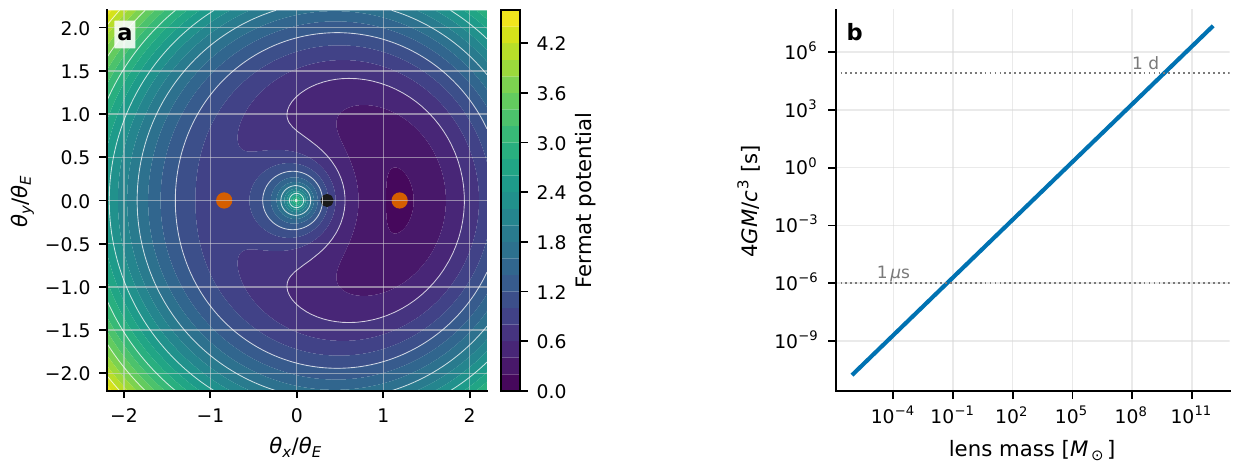
Figure 82 Two scales in strong lensing. The left panel shows the Fermat arrival-time surface for a point-mass lens. The black point is the source position and the two orange points are image positions; images appear at stationary points of the arrival-time surface. The right panel shows the basic delay scale 4GM/c³: stellar-mass lenses give microsecond to millisecond delays, while galaxy and cluster lenses naturally enter the day-to-year domain.

When wavelength cannot be ignored, the geometric-optics picture of separate rays must be replaced by a diffraction integral. For lensed gravitational waves, a common dimensionless frequency is

(284)\[w = \frac{8\pi GM(1+z_l)f}{c^3}.\]

For \(w\gg1\), geometric optics is recovered: multiple images can be separated and can produce coherent interference fringes. For \(w\lesssim1\), diffraction smooths caustics and the magnification can no longer be written as a simple sum of geometric images. In frequency space,

(285)\[\tilde h_L(f)=F(f)\,\tilde h(f),\]

where \(F(f)\) is a complex amplification factor. If two paths have delay \(\Delta t\), the approximate frequency spacing of interference fringes is

(286)\[\Delta f \simeq \frac{1}{\Delta t}.\]

For \(\Delta t=2\,{\rm ms}\), the fringe spacing is about \(500\,{\rm Hz}\). At electromagnetic optical frequencies, ordinary stellar or galaxy lenses usually have extremely large \(w\), so geometric optics is excellent. For LISA-band gravitational waves and \(10^6\)–\(10^9M_\odot\) lenses, wave-optics effects can enter the observing band [Takahashi and Nakamura, 2003].

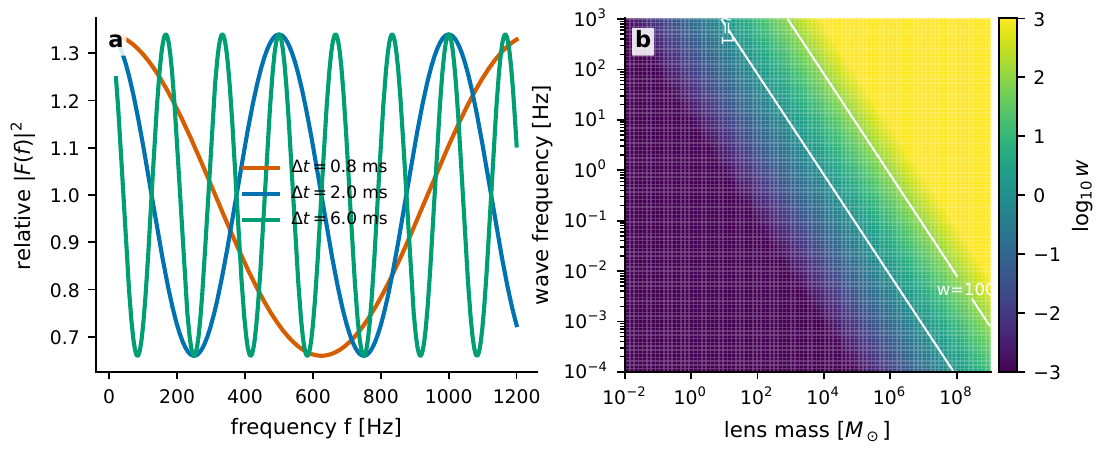
Figure 83 Wave-optics lensing turns time delay into frequency-domain fringes. The left panel shows relative-amplification oscillations for different path delays, with Δf ≃ 1/Δt. The right panel shows the scale of w = 8πGMf/c³. The white w = 1 contour marks the transition between diffraction and geometric optics; above w = 100, images can usually be treated as independent paths.

Correlation functions and the boundary of cosmic Bell tests

Multipath propagation rearranges intensity correlations. If a lens or scattering medium can be approximated by a set of discrete paths across the observing band,

(287)\[h(t)=\sum_i \sqrt{\mu_i}\,e^{i\varphi_i}\delta(t-t_i),\]

where \(\mu_i\) is the magnification of path \(i\), \(\varphi_i\) is its phase, and \(t_i\) is its arrival time. If phase is averaged over bandwidth or source size, the observed intensity is approximately

(288)\[I_{\rm obs}(t) = \sum_i \mu_i I_{\rm src}(t-t_i).\]

For intensity fluctuations \(\delta I=I-\langle I\rangle\), the autocorrelation function becomes

(289)\[C_{\rm obs}(\tau) = \left\langle \delta I_{\rm obs}(t)\, \delta I_{\rm obs}(t+\tau) \right\rangle = \sum_{ij}\mu_i\mu_j C_{\rm src}\!\left(\tau+t_i-t_j\right)\]

and can show echo structure near \(\tau=t_j-t_i\). This relation is useful only when the source itself has measurable fast structure, the propagation paths are stable, the observing time is long enough, and the background and selection function have been modeled. The \(g^{(2)}(0)\) peak of thermal light, giant-pulse microstructure in pulsars, narrow-band FRB scintillation, and lensed multiple image delays can all fit inside this framework. Their coherence times, bandwidths, and statistical distributions are different, so a correlation peak alone does not identify the physical origin.

Propagation effects also set the boundary conditions for cosmic Bell tests. A laboratory Bell test uses entangled photon pairs, with two stations choosing measurement settings \(a,a'\) and \(b,b'\). The CHSH combination is

(290)\[S = E(a,b)+E(a,b')+E(a',b)-E(a',b'), \qquad |S|\le 2\]

for any local-hidden-variable model. Cosmic Bell experiments use photons from Milky Way stars or high-redshift quasars in real time to choose \(a\) and \(b\). The purpose is to push possible common causes into an earlier spacetime region, not to prove that the astronomical photons themselves are entangled. The Milky-Way-star version used stellar color to generate settings while accounting for atmospheric delay, detector noise, and the probability of an incorrect setting. The quasar version pushed the possible shared past of the setting choices much farther back in cosmic history [Handsteiner et al., 2017, Rauch et al., 2018]. These experiments test causal structure. Astronomical photons can choose settings for a quantum-foundations experiment, but absorption, reddening, dispersion, and instrumental delay along their paths have to enter the timing model term by term.

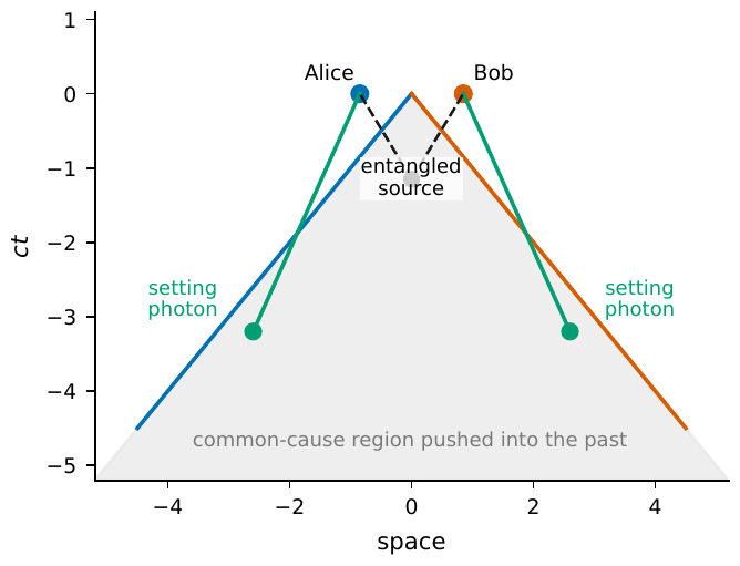
Figure 84 Light-cone structure of a cosmic Bell experiment. A local laboratory source emits entangled photon pairs, and Alice and Bob choose their measurement settings using photons from distant stars or quasars. The earlier and more widely separated those setting-photon emission events are, the larger the spacetime region excluded for possible common causes. The gray region marks the common-cause domain pushed into the past; real experiments must also include atmospheric propagation, detector response, and electronic delay.

Ordinary propagation effects set the error floor for searches for new physics. Axion-like particles can convert photons in magnetic fields, cosmic birefringence can rotate polarization, and dark-matter substructure can alter lensing magnification and time delay. Such explanations have to be compared in one model against plasma, dust, lensing, and instrumental terms. A residual signal becomes a serious new-physics candidate only if it survives tests in time, frequency, polarization, and angular position.