Teaching experiments and computational experiments#
Chapter opening
Observables, instrument response, and error budgets all return in the end to an event table. A tabletop HBT experiment, a uniform-disk fit, binary visibility, an event-table correlator, SPADE mode sorting, and a Type Ia supernova distance toy model look like different topics, but they all take the same kind of input: photon events carrying time, channel, polarization, and quality labels. The historical HBT foundation, quantum-optics teaching experiments, modern intensity-interferometry instruments, and mode-measurement ideas are discussed in Hanbury Brown [1956] [Abeysekara et al., 2020, Brown and Twiss, 1957, Glauber, 1963, Goodman, 1985, Kim et al., 2025, Ladera, 2002, Mandel and Wolf, 1995, Naletto et al., 2009, Nitu Rai et al., 2024, Sudarshan, 1963, Tsang et al., 2016].
Event tables and tabletop HBT#
The experiment starts with the event table; the mean light curve is only one projection of it. Each event row follows the fields in Eq. (1) of Chapter Mathematical and Physical Foundations, with detector identifier, quality flags, and timing corrections added according to the instrument-layer discussion in Chapter Detectors, clocks, and event tables. The file header should state whether times are stored in ns, ps, or GPS/UTC time stamps; how detector identifiers are encoded; whether spectral and polarization channels exist; and how quality flags mark events near dead time, clouds, electronic saturation, abnormal baselines, or background windows. Instruments such as AquEYE and Iqueye keep every photon as a time tag, with time resolution reaching tens of picoseconds and absolute timing usually constrained to ns or sub-ns scales by GPS, rubidium clocks, or White Rabbit-type synchronization systems [Jansweijer et al., 2013, Wahl et al., 2020, Zampieri et al., 2015, Zampieri et al., 2016]. Pixel-counting chips such as Timepix show that an event table can also carry spatial position, energy, or time-of-arrival information [Llopart et al., 2007].
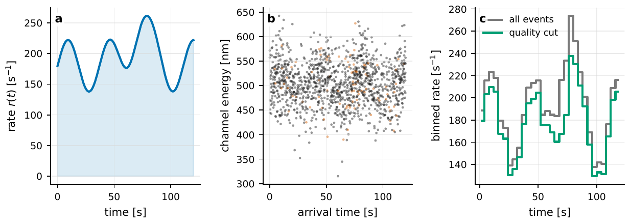
Figure 117 Simulated event table generated from an inhomogeneous Poisson process. The left panel shows the input photon rate r(t). The middle panel preserves individual photon arrival times, an effective wavelength channel, and quality flags. The right panel projects the event table into a light curve and shows the effect of quality selection. The event table retains channel and quality information that the light curve discards, so the same data can still be reused for correlation, polarization, or spectral analysis.#
If only a light curve is needed, the event table can be projected into time bins:
\(n_k\) is the photon count in bin \(k\) and is dimensionless. \(\Delta t\) is the bin width; tabletop experiments may use ns to ms bins, while astronomical timing can range from ns to minutes. \(q_i=1\) means that event \(i\) passes the quality selection. The rate estimate is \(r_k=n_k/\Delta t\), in \({\rm s}^{-1}\). When the mean count per bin is below a few to a few tens of photons, Poisson noise should not be replaced blindly by Gaussian error bars. Once \(n_k\gtrsim 30\), the Gaussian approximation is usually adequate. The unbinned Poisson point-process likelihood was given in Eq. (117), and the binned form in Eq. (118). The same event table can be fit directly in event time or after binning into a light curve; comparing the two shows how rapid variability and nonuniform exposure change the uncertainty. This is also why event-time segmentation methods such as Bayesian Blocks are useful for pulses, flares, and intensity-interferometry quality windows [Scargle et al., 2013].
Tabletop HBT experiments usually use thermal light, pseudothermal light, or a speckle source. A laser sent directly to two detectors gives \(g^{(2)}(0)\simeq1\). Pseudothermal light from a rotating ground glass can approach \(g^{(2)}(0)=2\) in the single-mode limit, while multimode light and finite time response reduce the peak [Adams et al., 2003, Banaszek et al., 1999, Banaszek and Wódkiewicz, 1996, Chen et al., 2011, Nitu Rai et al., 2024, Noh et al., 1991]. The delay histogram and \(g^{(2)}\) normalization were defined in Eqs. (120) and (122). A teaching experiment should make the user choose \(\Delta\tau\), time-shift background, and quality cuts explicitly. If \(R_1=R_2=5\times10^5\,{\rm s}^{-1}\), \(T=300\,{\rm s}\), and \(\Delta\tau=0.5\,{\rm ns}\), the accidental coincidences are about \(3.75\times10^4\) pairs per bin, with shot-noise fractional uncertainty \(1/\sqrt{H}\simeq5\times10^{-3}\). This order of magnitude is useful: a \(10^{-2}\) peak in \(g^{(2)}-1\) is visible on a tabletop, whereas a \(10^{-5}\) astronomical bunching peak requires large collecting area, long integration, and stable background.
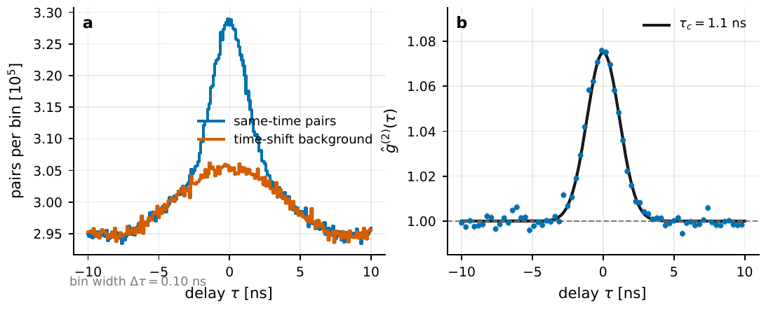
Figure 118 Delay histogram for a tabletop HBT experiment. The left panel compares same-time pairs with a time-shift background; slow drifts appear in both curves. The right panel normalizes by the background histogram to obtain ĝ(2)(τ). The width of the zero-delay peak is set jointly by the source coherence time and the detector response.#
A real instrument measures the ideal \(g^{(2)}\) convolved with the detector time response. Response convolution and the jitter budget were introduced in Eqs. (107) and (108). The report should state how the response kernel was measured, not only the final peak height. If the coherence time \(\tau_c\) is much shorter than the time bin or electronic response width \(\Delta t\), the observed thermal-light contrast is approximately diluted by \(\tau_c/\Delta t\). A visible narrowband filter centered at \(416\,{\rm nm}\) with a \(13\,{\rm nm}\) bandwidth has a coherence time of only order \(4\times10^{-14}\,{\rm s}\). With ns-scale electronics, the bunching contrast naturally falls to order \(10^{-5}\). VERITAS, MAGIC, and the Asiago photon-counting intensity-interferometry analyses all treat this dilution, together with background and dead time, explicitly [Abeysekara et al., 2020, Abe et al., 2024, Acharyya et al., 2024, Barbieri et al., 2009, Guerin et al., 2017, Karl et al., 2022, Naletto et al., 2009, Zampieri et al., 2021].
Uniform disks and binaries#
Once HBT is moved from the tabletop to two telescopes, the amplitude of the zero-delay peak in the delay histogram carries spatial-coherence information. The thermal-light Siegert relation was given in Eq. (16) of Chapter Mathematical and Physical Foundations; the spatial intensity-interferometry form was given in Eqs. (95) and (96) of Chapter Spatial coherence and intensity interferometry. \(\gamma_{12}\) is the first-order complex degree of coherence between the two telescopes, and \(|\gamma_{12}|^2\) is the normalized squared visibility of the source brightness distribution. \(\beta\) collects contrast dilution from time response, optical bandwidth, polarization selection, and instrument efficiency. If only one linear polarization is used and \(\tau_c/\Delta t=10^{-5}\), then \(\beta\) is commonly of order \(10^{-6}\)–\(10^{-5}\). A teaching simulation may deliberately set \(\beta=0.05\) so that the signal is visible, but the report must state that this is an artificial amplification.
The standard model for a disk-like star is the uniform disk in Eq. (6) of Chapter Mathematical and Physical Foundations and Eq. (93) of Chapter Spatial coherence and intensity interferometry; the first null is given in Eq. (94). \(\theta\) is angular diameter, in rad, mas, or \(\mu{\rm as}\). \(B_\perp\) is projected baseline, in m. \(\lambda\) is observing wavelength, in m. \(J_1\) is the first-order Bessel function. At \(\lambda=416\,{\rm nm}\), the first null for \(\theta=1\,{\rm mas}\) occurs near \(105\,{\rm m}\). This is why hundred-meter Cherenkov arrays such as VERITAS can measure bright-star diameters, whereas the few-\(\mu{\rm as}\) angular radii of Type Ia supernovae require kilometer-scale baselines.
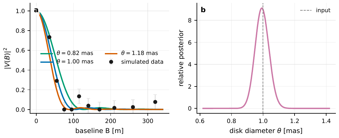
Figure 119 Uniform-disk intensity-interferometry fit. The left panel simulates |V|2 measurements for a \(\theta=1\,{\rm mas}\) target at \(\lambda=416\,{\rm nm}\). The slope is steepest near the first null, where the angular diameter is most strongly constrained. The right panel converts the data into an angular-diameter posterior; its width is set jointly by the |V|2 uncertainties, baseline coverage, and model assumptions.#
To estimate \(|V|^2\) from data, each baseline \(b\) first gives a zero-delay excess correlation \(\hat c_b=\hat g^{(2)}_b(0)-1\). A same-night calibrator or laboratory measurement gives the instrument contrast \(\beta_b\), and hence
Both \(\hat c_b\) and \(\hat\beta_b\) are dimensionless. If the accidental coincidence count is \(H_b\), and systematic terms are ignored for the moment, \(\sigma_{\hat c}\simeq H_b^{-1/2}\). Once \(\beta\) is as small as \(10^{-5}\), the same \(\sigma_{\hat c}\) is amplified into \(\sigma_{|V|^2}\simeq\sigma_{\hat c}/\beta\). A teaching simulation that uses an unrealistically large \(\beta\) will produce a beautiful \(g^{(2)}\) peak; astronomical \(|V|^2\) precision is still set by the true contrast, accidental coincidences, and systematic floor.
The binary model shows that although intensity interferometry loses the sign of the phase, spatial-frequency oscillations remain. The two-point-source \(|V|^2\) model was written in Eq. (175) of Chapter Stars as quantum light sources and Eq. (348) of Chapter First-generation quantum-astronomy science cases. The exercise only has to insert the flux ratio \(\rho=F_2/F_1\), angular separation vector \(\boldsymbol s\), and projected phase \(2\pi\boldsymbol B_\perp\cdot\boldsymbol s/\lambda\). \(\boldsymbol s\) is in radians, although reports usually quote it in mas. \(\boldsymbol B_\perp\cdot\boldsymbol s/\lambda\) is dimensionless. An equal-brightness binary with \(\rho=1\) can oscillate from 1 to 0. If the companion has only \(10\%\) of the primary flux, the modulation depth is about \(0.17\). At \(B=180\,{\rm m}\) and \(\lambda=500\,{\rm nm}\), a \(0.5\,{\rm mas}\) separation gives a phase of about 5.5, so even one baseline can see a clear oscillation. In orbital fitting, \(\boldsymbol s(t)\) changes with time, so a fixed baseline samples different phases.
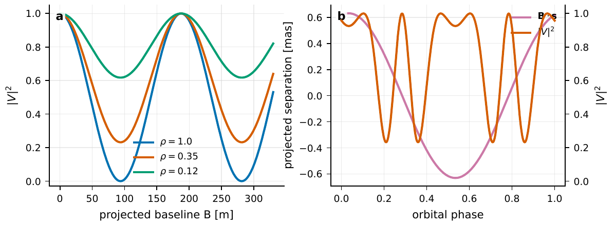
Figure 120 Binary |V|2 exercise. The left panel shows how the flux ratio ρ controls the depth of the baseline oscillation for a fixed angular separation. The right panel shows how the projected separation B ⋅ s changes with orbital phase in an inclined orbit, changing |V|2 on a fixed baseline. Multibaseline and multi-epoch data separate separation, flux ratio, and orbital geometry.#
Event-table correlators#
The correlator turns an event table into a set of delay histograms or covariance estimates. The most direct double loop compares all event pairs and scales as \(N_1N_2\). If the event lists are already sorted by time, only neighboring events within the correlation window \(|t_j-t_i|<\tau_{\max}\) need to be compared; the cost is roughly \(N_\gamma k\), where \(k\sim2R\tau_{\max}\) is the number of candidate events near each event. After projecting events onto uniform time bins, one can also compute cross-correlations with FFTs at cost \(M\log M\), where \(M=T/\Delta t\). These three routes estimate the same quantity, but they handle memory, time bins, and dead time differently.
For a many-telescope array, the number of baselines grows as \(N_{\rm tel}^2\), as in Eq. (99) of Chapter Spatial coherence and intensity interferometry: four telescopes have only 6 baselines, while 60 telescopes have 1770. The raw single-telescope data-rate estimate was given in Eq. (102) of Chapter Detectors, clocks, and event tables; for \(\Delta t=4\,{\rm ns}\), \(N_\nu=1\), and \(n_{\rm bit}=16\), \(D\simeq4\,{\rm Gb\,s^{-1}}\). If 64 spectral channels are kept, one telescope reaches \(256\,{\rm Gb\,s^{-1}}\). This explains why modern intensity interferometry needs GPU or FPGA real-time correlation, hierarchical triggering, on-chip accumulation, or strict data compression. The MAGIC real-time dead-time-free correlator and the VERITAS offline and online pipelines are both designed around this data-rate pressure [Abeysekara et al., 2020, Abe et al., 2024, Acharyya et al., 2024].
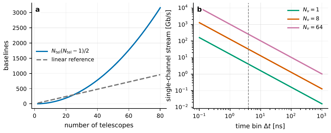
Figure 121 Two scaling laws for many-telescope correlators. The left panel shows the quadratic growth of baseline number with telescope count, so array expansion rapidly increases the number of correlation tasks. The right panel shows how a single data stream rises as time bins become narrower and spectral channels are added; ns sampling with tens of spectral channels already enters the regime where real-time hardware or GPU processing is needed.#
A correlator exercise must include null tests. If the second event stream is shifted by a time much longer than \(\tau_c\), the real peak should disappear. If the same pipeline is run with no starlight or with a shutter in place, electronic crosstalk should not create a zero-delay peak. If polarization or spectral channels are scrambled, only physically correlated channels should retain signal. If the data are split into time slices, \(\hat g^{(2)}(0)-1\) should converge as \(T^{-1/2}\), rather than being concentrated in one short interval. Experiments by Guerin and collaborators, AquEYE/Iqueye photon-counting schemes, and modern Cherenkov-array intensity interferometry all show that these quality controls determine whether the result can be interpreted [Abeysekara et al., 2020, Abe et al., 2024, Guerin et al., 2017, Zampieri et al., 2016, Zampieri et al., 2021].
Rayleigh curse and SPADE#
Direct imaging estimates the separation of two point sources from focal-plane pixel intensities. When the separation \(s\) of two equal-brightness incoherent point sources is much smaller than the point-spread-function width \(\sigma\), the image mostly broadens slightly. The derivative of the pixel intensities with respect to \(s\) approaches zero, so the Fisher information falls. This is the statistical meaning of the Rayleigh curse. Quantum estimation theory shows that the information has not disappeared from the optical field; it is stored in suitable spatial modes [Nair and Tsang, 2016, Tham et al., 2017, Tsang, 2015, Tsang et al., 2016].
For a Gaussian point-spread function and two equal-brightness point sources, the ideal Hermite–Gaussian mode-sorting probability was given in Eq. (142) of Chapter Quantum estimation, the Rayleigh limit, and sub-resolution information. The computational experiment treats \(n=0,1,2,\ldots\) as the transverse mode index and uses the same angular or focal-plane length unit for separation \(s\) and PSF width \(\sigma\). If \(s=0.2\sigma\), the dimensionless quantity that controls higher-mode weight is \(2.5\times10^{-3}\). Almost all photons still enter the \(n=0\) mode, but the small probability in \(n=1\) changes sensitively with \(s\). Ideal SPADE retains finite Fisher information for separation as \(s\to0\), whereas direct pixel imaging tends to zero. Experimentally, mode mismatch, centroid error, aberrations, and background introduce an information floor, so teaching code should include an adjustable mode-crosstalk parameter rather than plotting only the ideal curve.
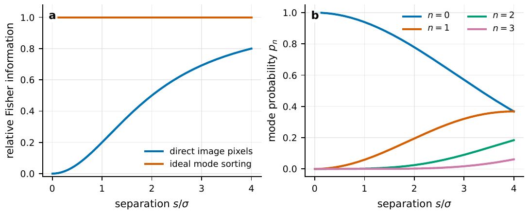
Figure 122 SPADE computational experiment. The left panel compares the relative Fisher information of direct pixel imaging and ideal mode sorting at small separation; direct imaging loses information for s/σ ≪ 1, while mode sorting remains nearly constant. The right panel shows Hermite–Gaussian mode probabilities. At small separation, higher-mode probabilities are tiny but have nonzero slope, so the measurement requires stable mode sorting and low crosstalk.#
This exercise and intensity interferometry point to the same lesson: conventional image resolution is not the information limit for every parameter. Intensity interferometry accesses long-baseline spatial frequencies through \(|V|^2\). SPADE accesses separation information that is barely visible in the direct image by projecting onto modes. Real astronomical systems face weak light, background, multimode mixing, turbulence, aberrations, and detector efficiency, so mode sorting is better treated as a computational experiment and pathfinder than as a promise that the next telescope will reach the quantum limit without loss.
Type Ia distance toy model and course projects#
The Type Ia supernova project combines several earlier exercises. A spectral model gives the photospheric velocity \(v_{\rm ph}(t)\). Intensity interferometry gives the angular photospheric radius \(\theta_{\rm ph}(t)\). Together they give an angular-diameter distance:
\(v_{\rm ph}\) is in \({\rm km\,s^{-1}}\); normal Type Ia supernovae are often at \(8000\)–\(15000\,{\rm km\,s^{-1}}\) at early times. \(t-t_0\) is in s or d, and intensity interferometry is most interested in the first days to weeks after explosion. \(D_A\) is usually quoted in Mpc. \(\theta_{\rm ph}\) is typically a few to a few tens of \(\mu{\rm as}\). For example, \(v_{\rm ph}=10^4\,{\rm km\,s^{-1}}\), \(t-t_0=15\,{\rm d}\), and \(D_A=20\,{\rm Mpc}\) give an angular radius of about \(4.3\,\mu{\rm as}\). At \(\lambda=500\,{\rm nm}\), \(\lambda/\theta\) corresponds to about \(24\,{\rm km}\). If the visibility curve is used rather than waiting for the first null, km to ten-km baselines still carry scientific information, but the error budget is tight [Kim et al., 2025].
The distance posterior can be written as
\(\hat\theta_k\) comes from the \(|V|^2\) fit at epoch \(k\), in \(\mu{\rm as}\) or radians. \(\hat v_k\) comes from spectral-line velocities or a radiation-transfer model, in \({\rm km\,s^{-1}}\). \(\sigma_{\theta,k}\) and \(\sigma_{v,k}\) include both statistical and model-systematic terms. A toy model that adds only \(10\%\) noise to \(\theta\) will produce an overly optimistic distance. A fuller project should let the explosion time \(t_0\), velocity gradient, asymmetry, and brightness-distribution model vary and then show how the posterior broadens.
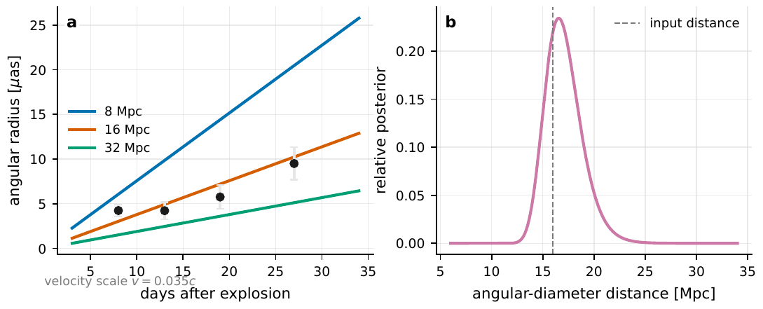
Figure 123 Type Ia supernova angular-diameter-distance toy model. The left panel uses a simplified expansion model with \(v_{\rm ph}=0.035c\) to show angular radius as a function of time for several distances, together with simulated angular-radius measurements. The right panel combines these radii with the velocity model to form a posterior for DA. A real analysis must replace the constant-velocity shell with a radiation-transfer model and include asymmetry, line-forming layers, and baseline coverage in the error budget.#
Course projects can be arranged by difficulty. The simplest experiment uses an LED, pseudothermal light, and a laser to measure \(g^{(2)}(\tau)\), reporting \(R_1\), \(R_2\), \(T\), \(\Delta\tau\), \(\tau_c\), and the response kernel \(K\). The same event table can then be used to implement time-shift background, quality cuts, and a \(T^{-1/2}\) convergence test. After moving to spatial coherence, students can fit uniform-disk and binary \(|V|^2\), and compare how baseline coverage changes the constraints on \(\theta\), \(\rho\), and \(\boldsymbol s\). A more information-theoretic project implements SPADE probabilities and Fisher information, with mode crosstalk and centroid error. An integrated project can build the Type Ia distance toy model and propagate angular-radius, velocity, and explosion-time uncertainties together. Each project should produce an event-table description, a Python script, a set of PDF figures, a short report citing ADS BibTeX keys, and at least two null tests.
Running code is only the first requirement. A timing-correlation project must state the time reference, bin width, dead time, dark counts, and accidental coincidence estimate. A spatial-coherence project must state \(B_\perp\), \(\lambda\), \(\beta\), \(|V|^2\) calibration, and source model. A mode measurement project must state the point-spread-function width, mode basis, crosstalk matrix, and background. A distance project must state the angular-radius estimate, velocity model, explosion time, and systematic error. Without these quantities, the figures may still render, but the result is not an astronomical measurement.