First-generation quantum-astronomy science cases#
Chapter opening
First-generation science cases must satisfy several constraints at once: photon rate, angular scale, baseline coverage, calibration difficulty, and a useful scientific outcome even if the most ambitious detection fails. Intensity interferometry has already moved from the Sirius experiment and the Narrabri stellar angular diameters to VERITAS, MAGIC, photon-counting observations of Vega, and recent measurements of rapid stellar rotation. Those results point to the same starting region: bright, hot, small-angular-scale targets with strong external priors. Stellar angular diameters, rapid rotation, close binaries, Be and Wolf–Rayet line-forming regions, early nova expansion, Crab photon statistics, and astrophysical-laser candidates form the most realistic first project list [Abeysekara et al., 2020, Abe et al., 2024, Acciari et al., 2020, Dravins et al., 2012, Hanbury Brown, 1956, Hanbury Brown et al., 1974, Le Bohec and Holder, 2006, Zampieri et al., 2021].
Case ranking starts with three coordinates#
Brightness is the first gate. For present intensity interferometry, \(m_V\lesssim5\) hot stars are the validation regime, \(m_V\simeq6-7\) is challenging but still plannable, and \(m_V\gtrsim9\) usually requires a larger array, multiple spectral channels, long integrations, or lower systematic noise. The target studies by Dravins and collaborators naturally place bright hot stars, emission-line structures, and rapid rotators at the beginning. The LeBohec–Holder estimate also shows that a pair of \(100\,{\rm m^2}\) telescopes with GHz electronic bandwidth can reach a few-sigma correlation detection in 5 h for an \(m_V\simeq6.7\) source [Dravins et al., 2010, Dravins et al., 2012, Dravins et al., 2013, Le Bohec and Holder, 2006].
Angular scale decides whether those photons become parameter constraints. If the target scale \(\theta\) is much larger than \(\lambda/B\), then \(|V|^2\) on long baselines is nearly zero and only short baselines retain signal. If \(\theta\) is much smaller than \(\lambda/B\), all baselines see an unresolved source and the diameter derivative is weak. The best first projects place the main structure on the 50–300 m baselines of existing IACTs or on the 0.5–2 km baselines of future CTA-like arrays. External priors also change how interpretable the data are. Known distance, spectrum, orbit, radial velocity, calibrator diameter, or theoretical model can turn a small number of \(|V|^2\) measurements into physical parameters [Jensen et al., 2010, Monnier, 2003, Nuñez et al., 2012, Nuñez et al., 2012, Nuñez et al., 2010].
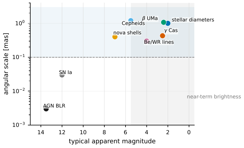
Figure 111 Brightness and angular scale of first-generation candidate targets. Bright-star diameters, β UMa, γ Cas, and Be/WR line-forming regions are both bright enough and large enough to be resolved on hundred-meter baselines. Type Ia supernovae, AGN broad-line regions, and small-scale dark lensing have high scientific value, but their brightness, event rate, or angular scale moves them into the longer-term category.#
A practical priority score can be written as
\(W_{\rm sci}\) is scientific return, \(R_{\rm tech}\) is technical maturity, \(R_{\rm prior}\) is the value of external priors and model interpretability, \(R_{\rm sys}\) is systematic-error risk, and \(R_{\rm trigger}\) is trigger and scheduling risk. In practice, a coarse score is enough. Its purpose is to keep one attractive dimension from dominating the decision. A Type Ia geometric-distance program has very high \(W_{\rm sci}\), but also high \(R_{\rm trigger}\) and \(R_{\rm tech}\). Bright-star angular diameters have more modest \(W_{\rm sci}\), but high \(R_{\rm tech}\) and low systematic risk, which makes them suitable first-generation acceptance tests [Abe et al., 2024, Acharyya et al., 2024, Kim et al., 2025].
Stellar diameters, effective temperatures, and rapid rotation#
Angular diameter is the most mature first-generation product. The observable is \(|V|^2(B,\lambda)\). The model usually starts with a uniform disk and then adds a limb-darkened profile or a full atmosphere model. The route from angular diameter to effective temperature is direct:
\(F_{\rm bol}\) is the bolometric flux received at Earth, in \({\rm W\,m^{-2}}\). \(\theta_{\rm LD}\) is the limb-darkened angular diameter, in radians. \(\sigma_{\rm SB}\) is the Stefan–Boltzmann constant. A \(4\%\) uncertainty in \(\theta_{\rm LD}\) propagates into only about a \(2\%\) uncertainty in \(T_{\rm eff}\) from the diameter term alone. Repeated bright-star diameter measurements are therefore not only instrument reproducibility tests; they enter the calibration of \(T_{\rm eff}\), radius, age, rotation models, and standard-star scales [Blackwell and Shallis, 1977, Davis and Tango, 1986, Hanbury Brown et al., 1974, Hanbury Brown et al., 1967, Monnier, 2003].
VERITAS-SII has already moved this program into a modern instrument setting. It measured sub-milliarcsecond diameters for \(\beta\) CMa and \(\epsilon\) Ori, reaching better than \(5\%\) precision with much less observing time than Narrabri. The later \(\beta\) UMa observation at 416 nm obtained a limb-darkened diameter \(\theta_{\rm LD}=1.07\pm0.04_{\rm stat}\pm0.05_{\rm sys}\,{\rm mas}\), in agreement with CHARA near-infrared and Keck mid-infrared measurements. The upgraded MAGIC-SII system reported 22 stellar diameters, including 9 reference stars and 13 stars without comparable previous measurements. Intensity interferometry is now beginning to provide diameter samples, not only isolated demonstrations [Abeysekara et al., 2020, Abe et al., 2024, Acharyya et al., 2024].
Rapid rotators are the natural next step beyond angular diameter. A uniform disk needs only \(\theta\). An elliptical photosphere needs at least a minor axis \(\theta_{\rm min}\), an axial ratio \(r=\theta_{\rm maj}/\theta_{\rm min}\), and a position angle \(\varphi_\star\). The elliptical visibility model can be written as
\(\psi\) is the angle of the projected baseline relative to the minor axis. If the baseline position-angle coverage is poor, \(r\) and \(\varphi_\star\) are strongly degenerate. The VERITAS result for \(\gamma\) Cas gives a minor-axis angular diameter of about \(0.43\pm0.02_{\rm stat}\pm0.02_{\rm sys}\,{\rm mas}\), an axial ratio of about \(1.28\pm0.04\pm0.02\), and a rotation-axis position angle of about \(116^\circ\). A Roche–von Zeipel model then implies rotation near the critical rate. First-generation intensity interferometry can therefore move from size to shape and gravity darkening [Archer et al., 2025].
Binaries, Be-star disks, and Wolf–Rayet winds#
Close binaries are attractive because their signal has a recognizable shape. For two unresolved point sources with angular-separation vector \({\bf s}\) and flux ratio \(f=F_2/F_1\),
\({\bf u}={\bf B}_\perp/\lambda\). For \(f=1\), \(|V|^2\) oscillates from 1 to 0. For \(f=0.1\), the modulation amplitude is only \(2f/(1+f)^2\simeq0.17\), so calibration and SNR requirements become much tighter. Binary projects are best suited to systems with existing spectroscopic or eclipsing-binary priors. A small number of baseline points per night can then be tied together by the orbital model, and a nondetection still gives an upper limit on separation or flux ratio [Hanbury Brown et al., 1974, Karl et al., 2022, Malvimat et al., 2014, Nuñez et al., 2012].
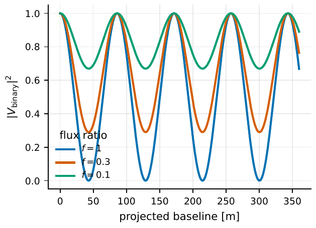
Figure 112 Squared-visibility oscillations for a 1 mas binary at 416 nm. An equal-brightness binary gives deep oscillations; once the flux ratio falls to 0.3 or 0.1, the modulation shrinks quickly. Binary programs need baseline coverage and orbital priors, otherwise flux ratio, separation, and position angle become mutually degenerate.#
Be-star disks and Wolf–Rayet winds connect spatial resolution with spectral selection. The continuum mainly comes from the photosphere, while H\(\alpha\), He, or Fe lines may come from an extended disk, a wind-collision region, or dense structures such as the Weigelt blobs. If line and continuum are mixed, the observed visibility is a flux-weighted sum:
\(F_{\rm line}/F_{\rm c}\) can be estimated from simultaneous spectroscopy or from narrowband and continuum filters. If the line-forming region is larger than the photosphere, \(|V_{\rm line}|^2\) falls faster on long baselines than the continuum. If the line comes from a compact bright clump, long baselines retain signal. Narrabri observations of the WR wind in \(\gamma^2\) Velorum already showed that emission-line and continuum regions can have different angular scales. Modern multibaseline arrays can extend the same idea to Be decretion disks, rapidly rotating hot stars, and interacting binaries [Archer et al., 2025, Dravins et al., 2010, Dravins et al., 2012, Hanbury Brown et al., 1970].
Novae, Type Ia supernovae, and triggered transients#
The geometry of an expanding transient is simple, but the observing requirements are hard. If a shell expands approximately freely with velocity \(v_{\rm exp}\), its angular diameter is
\(v_{\rm exp}\) comes from spectral-line velocities, in \({\rm m\,s^{-1}}\). \(D\) is distance, and \(t-t_0\) is time since explosion. A Galactic nova at \(D=2\,{\rm kpc}\) with \(v_{\rm exp}=1000\,{\rm km\,s^{-1}}\) reaches an angular diameter of several milliarcseconds after 10 days and can be resolved on sub-hundred-meter baselines. The main difficulties are brightness evolution, nonspherical structure, and dust. A Type Ia supernova at \(D=10\,{\rm Mpc}\) with \(v_{\rm exp}=10^4\,{\rm km\,s^{-1}}\) has an angular diameter of only \(\sim0.02\,{\rm mas}\) after 20 days, requiring kilometer-scale optical baselines. The limiting factors are trigger window, brightness, and array size [Kim et al., 2025].
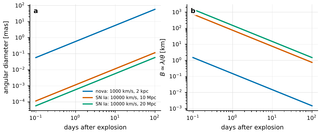
Figure 113 Angular diameter and required baseline for expanding transients. Galactic novae reach milliarcsecond scales within days to weeks, making them good first-generation trigger exercises. Type Ia supernovae at 10–20 Mpc remain at tens of microarcseconds even near peak, requiring kilometer baselines and nearby events with m ≲ 12.#
Type Ia intensity-interferometry distances are a high-return long-term target. The feasibility study by Kim et al. treats \(m\lesssim12\) as the brightness range for a foreseeable next-generation observation, corresponding to the local volume at \(z\sim0.004\) and roughly one usable Type Ia event per year over the whole sky. They used radiation-transfer models to compute surface-brightness profiles and \(|V|^2\) at different wavelengths, and showed that spectral resolution can provide multiwavelength tomography rather than a single uniform-disk radius. First-generation programs should practice triggering, filtering, background control, and model fitting with novae and nearby bright transients. A Type Ia distance scale belongs to a second-generation or dedicated-array program [Fouque and Gieren, 1997, Kim et al., 2025, Storm et al., 2004].
Crab photon statistics and astrophysical lasers#
The Crab pulsar is not the best target for spatial intensity interferometry, but it is an excellent event-table target. It is bright, has a stable period, and has an accurate ephemeris, so the optical main pulse and interpulse define phase windows. A timing error gives a phase error
For the Crab, \(P_{\rm spin}\simeq33\,{\rm ms}\), so a \(1\,\mu{\rm s}\) timing error gives only \(\Delta\phi\simeq3\times10^{-5}\). Millisecond pulsars are more demanding. Instruments such as AquEYE and Iqueye already store photons with picosecond to nanosecond time tags, which makes them suited to phase-resolved \(g^{(2)}\), color correlations, or conditional stacking on radio giant pulses. Optical enhancement during Crab giant-radio-pulse periods has been measured, and ARCONS found stronger optical enhancement for earlier giant pulses. First-generation quantum astronomy can translate these results into event-table statistics and polarization or color windows instead of stopping at mean light curves [Barbieri et al., 2009, Naletto et al., 2009, Shearer et al., 2003, Strader et al., 2013, Zampieri et al., 2015].
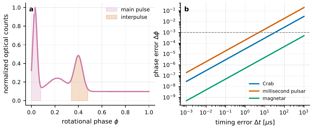
Figure 114 Phase windows and timing errors for a Crab-like optical pulse. The left panel sketches event selections for the main pulse, bridge, and interpulse. The right panel converts timing error into phase error. Microsecond timing is already generous for the Crab; for millisecond pulsars, ns–μs synchronization is needed to preserve narrow phase structure.#
Astrophysical-laser and stimulated-emission candidates are best treated as tests of nonthermal photon statistics; a bright spectral line alone is not enough. For \(M\) mutually incoherent thermal modes,
whereas an ideal coherent state gives \(g^{(2)}(0)=1\). Unsaturated maser/laser emission, saturated amplification, spontaneous background, multiple unresolved clumps, and instrument time response all produce different statistics. Fe II lines in the Weigelt blobs of Eta Carinae are pumped by Ly\(\alpha\); Johansson and Letokhov discussed Fe II laser lines at \(0.9-1.0\,\mu{\rm m}\) and in the near-infrared. Line-width measurements and photon-correlation spectroscopy can provide direct evidence. If the line width is \(\Delta\nu\), the coherence time is roughly \(\tau_c\sim1/(\pi\Delta\nu)\). A narrow line greatly improves resolvable correlation contrast for a given detector time resolution, but it also demands higher spectral resolution, stable filtering, and strict continuum subtraction [Dravins and Germanà, 2008, Johansson and Letokhov, 2004, Johansson and Letokhov, 2005].
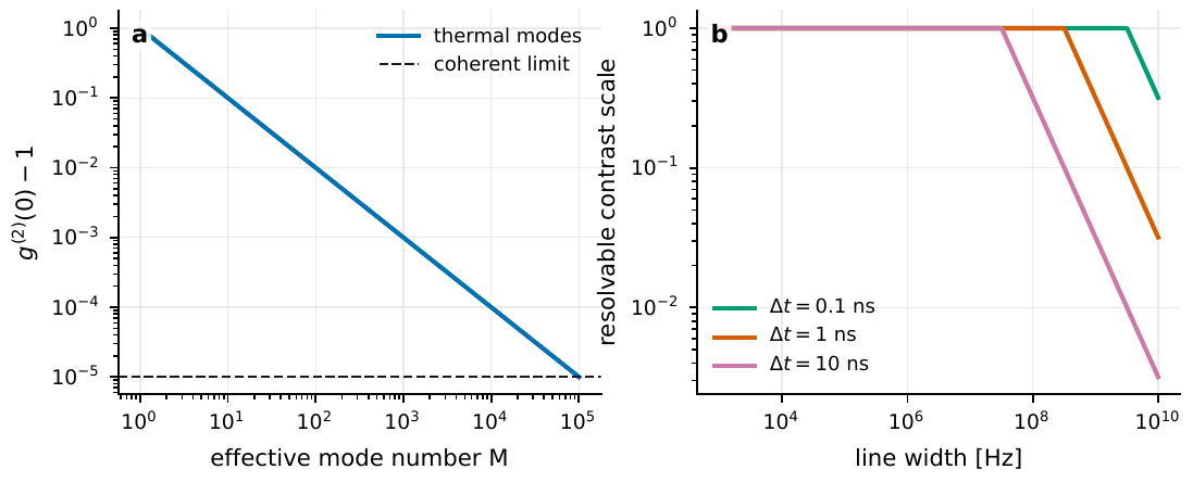
Figure 115 Two statistical quantities for astrophysical-laser candidates. The left panel shows how increasing the number of thermal modes suppresses the bunching peak, while the coherent limit approaches g(2)(0) − 1 = 0. The right panel shows that narrower lines have longer coherence times and therefore retain more resolvable contrast at fixed detector time resolution.#
Recommended first-generation sequence#
Putting these cases into one matrix, the first-generation order is set mainly by maturity and systematic risk. Bright hot-star diameters, known-diameter reference stars, \(\beta\) UMa-like A stars, and repeatable MAGIC/VERITAS targets are the best acceptance tests. \(\gamma\) Cas-like rapid rotators, Be/WR line-forming regions, close binaries, and early nova expansion add more scientific information on top of the same basic capability. Phase-resolved Crab statistics and astrophysical-laser candidate lines depend more strongly on event-table quality and timing or spectral cuts. Type Ia geometric distances, AGN broad-line regions, small-scale dark-matter lensing, and quantum-network-assisted imaging have high scientific return, but they belong in the longer-term program.
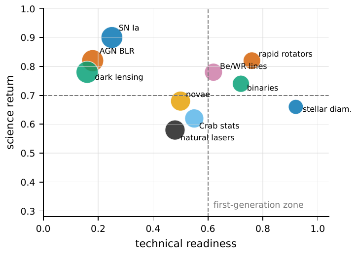
Figure 116 Matrix of first-generation science cases. The horizontal axis is technical maturity, the vertical axis is scientific return, and larger points indicate higher systematic and trigger risk. Targets in the upper-right region with smaller points are best suited for first-generation validation; upper-left targets are scientifically valuable but require dedicated arrays or more mature quantum resources.#
Case |
First observable |
Typical scale |
First-generation criterion |
|---|---|---|---|
Bright-star diameters |
$ |
V |
^2(B)$ |
Rapid rotators |
Multi-position-angle $ |
V |
^2$ |
Binaries |
$ |
V |
^2$ oscillations |
Be/WR lines |
Line/continuum $ |
V |
^2$ |
Novae |
\(\theta(t)\) |
Milliarcsecond scale after a few days |
Fast trigger and combination with line velocities. |
Crab statistics |
Phase-window \(g^{(2)}\) and color correlations |
\(P=33\,{\rm ms}\) |
Closure of ephemeris, nebular background, and absolute timing. |
Astrophysical lasers |
\(g^{(2)}\), line width, polarization |
\(\Delta\nu\) can be narrow enough for long coherence time |
Separable line and continuum, with a null test. |
Type Ia |
$ |
V |
^2(\lambda,t)$ |
The ranking changes as the instrument changes. When timing synchronization and zero-baseline correlations have just been closed, bright-star diameters and reference-star repeatability are the most valuable tests. Once six or more baselines run reliably, rapid rotators and binaries move into the main list. Once narrowband filtering and high data throughput are reliable, astrophysical lasers and line-forming disks become realistic. When the array reaches kilometer scales and can respond rapidly to \(m\lesssim12\) transients each year, Type Ia geometric distances become front-line science [Abe et al., 2024, Acharyya et al., 2024, Archer et al., 2025, Guerin et al., 2017, Karl et al., 2022, Kim et al., 2025].