Photon statistics and coherence functions

Chapter opening

The previous chapters described telescope data as labelled detection events. Photon statistics asks the next question: do those events arrive independently, or do they carry measurable joint structure across time delay, frequency separation, polarization combination, or spatial channel? This question began with the Hanbury Brown–Twiss experiments, Glauber’s coherence theory, and Mandel’s photon-counting theory. It is now shared language for quantum optics and modern astronomical intensity interferometry [Brown and Twiss, 1956, Brown and Twiss, 1957, Brown and Twiss, 1958, Fano, 1961, Glauber, 1963, Glauber, 1963, Goodman, 2000, Mandel and Wolf, 1965, Mandel and Wolf, 1995, Wolf, 2007].

From event tables to counts and factorial moments

Write the event table for detection channel \(j\) as

\[\mathcal{D}_j=\{t_{j,q},\nu_{j,q},p_{j,q},w_{j,q}\}_{q=1}^{N_j}.\]

\(t_{j,q}\) is the arrival time, usually in seconds. \(\nu_{j,q}\) is the frequency or band in which the photon was recorded. \(p_{j,q}\) is a polarization or detector-channel label. \(w_{j,q}\) is a quality weight, such as a dead-time correction, a background probability, or a bad-pixel mask. Optical HBT and intensity-interferometry measurements often work with nanosecond electronic response. X-ray and gamma-ray event tables may have microsecond to millisecond time stamps. Ordinary imaging or spectroscopy, if it stores only integrated pixel intensities, has already averaged over much of the timing information.

For a time gate \([t_k,t_k+\Delta t)\), the count is

(70)\[N_{j,k}(\Delta t)=\sum_q w_{j,q}\, \mathbf{1}\!\left(t_k\leq t_{j,q}<t_k+\Delta t\right), \qquad \widehat r_{j,k}=\frac{N_{j,k}}{\Delta t}.\]

\(N_{j,k}\) is dimensionless. \(\widehat r_{j,k}\) has units \(\mathrm{s^{-1}}\). If \(\Delta t=1\,\mathrm{ns}\) and the mean photon rate is \(10^6\,\mathrm{s^{-1}}\), the mean count in one gate is only \(10^{-3}\). Most bins are zero, a small fraction contain one photon, and two photons in the same bin are rare. Correlations are therefore not read off by eye from a light curve. They are accumulated over \(10^8\)–\(10^{12}\) time gates or event pairs.

Second-order counting uses the factorial moment, not the ordinary second moment \(\langle N^2\rangle\):

(71)\[\left\langle N(N-1)\right\rangle.\]

\(N^2\) includes the unphysical pairing of a photon with itself. \(N(N-1)\) counts ordered pairs made from distinct photons. Photoelectric coincidence counting has exactly this structure: one START photon and one STOP photon form a pair; a single detector pulse does not trigger itself twice. Glauber’s normally ordered operators build this fact into the theoretical definition, while Mandel’s counting theory builds it into the measured count distribution [Glauber, 1963, Glauber, 1963, Mandel and Wolf, 1965].

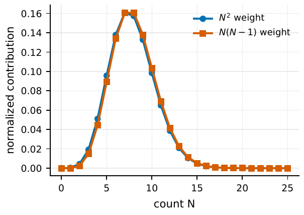
Figure 18 In a Poisson count distribution, the ordinary moment N² and the factorial moment N(N − 1) weight each count value differently. Coincidence detection cares about photon pairs made from distinct photons, so N(N − 1) automatically removes self-pairing.

A single-channel autocorrelation is often measured by splitting the beam and cross-correlating two detectors. The reason is instrumental. Avalanche photodiodes, photomultipliers, and other single-photon detectors have dead time. If a detector cannot respond for \(10\)–\(100\,\mathrm{ns}\) after a trigger, a single-detector autocorrelation develops an artificial hole near zero delay. Sending the same beam through a 50:50 beamsplitter to two independent detectors separates the photon statistics of the light from the recovery time of one detector. Guerin et al. used exactly this architecture for stellar thermal-light bunching with 1 m telescopes: multimode fiber, beamsplitter, two APDs, and a TDC delay histogram. Their APD dead time was about \(22\,\mathrm{ns}\), whereas the optical coherence time was at the picosecond scale. Without the beamsplitter, the zero-delay peak would have been hard to measure [Guerin et al., 2017].

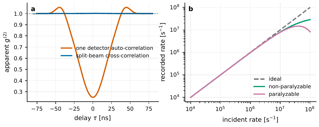
Figure 19 How dead time, pile-up, and afterpulsing affect short-delay correlations. The left panel shows that a single-detector autocorrelation can develop a zero-delay hole and false peaks at nonzero delay, while a split-beam two-detector cross-correlation is closer to the true thermal bunching peak. The right panel shows how different dead-time models produce different recorded-rate saturation curves at high incident photon rate.

Quantity	Units and typical range	Physical meaning
\(t_{j,q}\)	s; timing precision from ns to ms	Arrival time of one detection event; differences between event times form the delay axis of a correlation function.
\(\Delta t\)	ps to s	Chosen count gate or electronic sampling interval; if it is much longer than the coherence time, it dilutes the bunching peak.
\(r_j\)	\(\mathrm{s^{-1}}\); optical HBT often uses \(10^5\)–\(10^7\)	Mean count rate in channel \(j\), which sets shot noise and the number of available event pairs.
\(\tau_d\)	ns to \(\mu\mathrm{s}\)	Detector dead time; if it is comparable to the delays of interest, one needs beam splitting, cross-correlation, or a dead-time model.
\(H_{AB}(\tau)\)	counts per delay bin	Delay histogram of event pairs from two channels; after normalization it gives \(g^{(2)}\).

First-order and second-order coherence

At the detector plane, write the positive-frequency electric-field operator as \(\hat E^{(+)}(t)\), with negative-frequency part \(\hat E^{(-)}(t)\). The first-order coherence function is

(72)\[G^{(1)}(t_1,t_2) = \left\langle \hat E^{(-)}(t_1)\hat E^{(+)}(t_2) \right\rangle, \qquad g^{(1)}(\tau)=\frac{G^{(1)}(t,t+\tau)}{G^{(1)}(t,t)} .\]

\(G^{(1)}\) carries intensity units, while \(g^{(1)}\) is dimensionless. For a stationary field, the correlation depends only on the delay \(\tau=t_2-t_1\). \(|g^{(1)}|\) measures how much the electric-field phase is remembered after delay \(\tau\). In an amplitude interferometer it directly sets the fringe visibility. Narrower spectra give longer coherence times. For a filter with central wavelength \(\lambda\) and bandwidth \(\Delta\lambda\ll\lambda\),

(73)\[\Delta\nu \simeq \frac{c\,\Delta\lambda}{\lambda^2}, \qquad \tau_c \sim \frac{1}{\Delta\nu} \simeq \frac{\lambda^2}{c\,\Delta\lambda}.\]

At \(\lambda=780\,\mathrm{nm}\) with \(\Delta\lambda=1\,\mathrm{nm}\), \(\tau_c\) is about \(2\,\mathrm{ps}\). Broad optical filters usually give a thermal-light coherence time far shorter than a nanosecond detector response. This scale recurs in stellar bunching experiments, photon-correlation spectroscopy of narrow astrophysical lines, and the later discussion of spatial coherence and intensity interferometry [Dravins and Germanà, 2008, Foellmi, 2009, Guerin et al., 2017].

The second-order coherence function asks whether two intensity detections occur together more often than random arrivals would predict:

(74)\[G^{(2)}(t_1,t_2) = \left\langle \hat E^{(-)}(t_1)\hat E^{(-)}(t_2) \hat E^{(+)}(t_2)\hat E^{(+)}(t_1) \right\rangle, \qquad g^{(2)}(\tau)= \frac{G^{(2)}(t,t+\tau)} {G^{(1)}(t,t)\,G^{(1)}(t+\tau,t+\tau)} .\]

\(g^{(2)}\) is dimensionless. Independent Poisson arrivals give \(g^{(2)}=1\). If \(g^{(2)}(0)>1\), neighboring photons are bunched; one ideal thermal space-time-polarization mode has \(g^{(2)}(0)=2\). If \(g^{(2)}(0)=1\), the arrival times are second-order Poisson-like, as for a coherent state. If \(g^{(2)}(0)<1\), zero-delay coincidences are suppressed. This is antibunching, the standard criterion for single-photon sources and resonance fluorescence in quantum optics, and it cannot be described by a positive classical intensity fluctuation [Birnbaum et al., 2005, Kimble et al., 1977, Mandel, 1979, Yurke et al., 1986, Żukowski et al., 1993].

The continuous-intensity form

(75)\[g^{(2)}(\tau)= \frac{\left\langle I(t)I(t+\tau)\right\rangle} {\left\langle I(t)\right\rangle^2}\]

is useful for estimates, but it hides normal ordering and detector response. \(I(t)\) may mean ideal instantaneous intensity, detector output current, a TDC event rate, or a sampled ADC trace. If \(I(t)\) has already been convolved with a \(4\,\mathrm{ns}\) electronic response, the result is the response-broadened \(g^{(2)}\), not the picosecond-wide correlation peak of the optical field. In astronomical data analysis this distinction matters: the area of the true bunching peak may be preserved while its height is suppressed by three to six orders of magnitude.

Mandel \(Q\), thermal light, multimode light, and antibunching

Let \(N\) be the count in a fixed time gate, with mean \(\bar{N}\) and variance \(\sigma_N^2\). Mandel’s parameter is

(76)\[Q=\frac{\sigma_N^2-\bar{N}}{\bar{N}}.\]

\(Q=0\) denotes Poisson counts. \(Q>0\) means that the variance exceeds shot noise. \(Q<0\) means sub-Poisson counts. For zero-delay second-order coherence inside the same gate,

(77)\[g^{(2)}(0)= \frac{\left\langle N(N-1)\right\rangle}{\bar{N}^2} = 1+\frac{Q}{\bar{N}}.\]

Here \(N\) is the count in one gate, not the total count in the whole observation. If the gate width is increased, \(\bar{N}\) increases and many mutually incoherent time modes are averaged together. Even for intrinsically thermal light, the observed value of \(g^{(2)}(0)-1\) then falls.

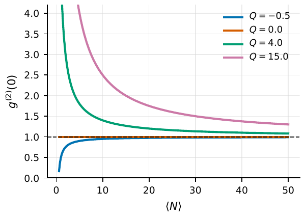
Figure 20 Within a fixed time gate, Mandel Q shifts the zero-delay coherence through g⁽²⁾(0) = 1 + Q/⟨N⟩. At low mean count, the same Q produces a larger departure from g⁽²⁾(0) = 1. Averaging many modes drives the curve back toward unity.

Single-mode thermal light has a Bose–Einstein count distribution,

(78)\[P(N)=\frac{\bar{N}^{\,N}}{(1+\bar{N})^{N+1}}, \qquad \sigma_N^2=\bar{N}+\bar{N}^2, \qquad g^{(2)}(0)=2.\]

The \(\bar{N}^2\) term is wave noise, and the \(\bar{N}\) term is shot noise. Astrophysical thermal radiation has this statistic in a sufficiently narrow single space-time-polarization mode, but real telescopes usually collect many independent modes at once. If \(M\) independent thermal modes of comparable intensity are averaged by the same detector, the variance becomes

(79)\[\sigma_N^2=\bar{N}+\frac{\bar{N}^2}{M}, \qquad g^{(2)}(0)=1+\frac{1}{M}.\]

\(M\) may come from two polarizations, many spatial speckles, many frequency modes inside a broad bandpass, or many coherence times inside one analysis gate. For an unresolved-polarization thermal point source, \(M_{\rm pol}\) is already about 2, so the ideal peak falls from 2 to 1.5. If \(\Delta t/\tau_c=10^3\), time averaging reduces the excess by another factor of roughly \(10^3\).

A coherent state gives Poisson counts:

(80)\[P(N)=e^{-\bar{N}}\frac{\bar{N}^N}{N!}, \qquad \sigma_N^2=\bar{N}, \qquad g^{(2)}(\tau)=1.\]

An ideal laser can have a long first-order coherence time without producing thermal bunching in second-order intensity fluctuations. In astronomy the phrase “coherent emission” needs care. Radio masers, coherent curvature radiation in pulsars, candidate astrophysical laser lines, and nonthermal synchrotron emission can differ in first-order coherence, second-order coherence, and multi-source averaging. Many astrophysical masers are sums over many small coherence cells, so the observed \(g^{(2)}\) need not resemble a laboratory single-mode laser [Cheng and Ruderman, 1977, Dravins and Germanà, 2008, Foellmi, 2009, Johansson and Letokhov, 2004, Johansson and Letokhov, 2005, Johansson and Letokhov, 2005, Michel, 1991].

The Siegert relation and its boundaries

Thermal light, and more generally chaotic Gaussian light, has a useful simplification: fourth-order field correlations factor into products of second-order field correlations. After normalization this gives the Siegert relation

(81)\[g^{(2)}(\tau)=1+\zeta\left|g^{(1)}(\tau)\right|^2 .\]

\(\zeta\) is a visibility factor with \(0<\zeta\leq1\). An ideal single space-time-polarization mode has \(\zeta=1\). Unresolved polarization, multiple spatial modes, finite-bandwidth averaging, background light, and instrumental response all lower \(\zeta\). If source photons make up fractions \(f_A\) and \(f_B\) of the total count rates in two channels, and if the background is uncorrelated and has no bunching signal of its own, the correlation-peak amplitude is approximately multiplied by \(f_A f_B\).

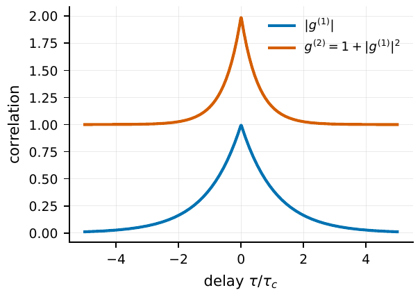
Figure 21 For thermal light, the Siegert relation turns the decay of first-order field coherence into a second-order intensity-bunching peak. If |g⁽¹⁾| decays with coherence time τ_c, then g⁽²⁾ − 1 decays as |g⁽¹⁾|² and returns to zero at large delay. In a real instrument, the peak height is further multiplied by mode-number, background, and timing-response factors.

The left-hand side of Eq. (81) can be estimated from an event table. The \(g^{(1)}\) on the right-hand side can be obtained from the Fourier transform of the spectrum, or measured as visibility in an amplitude interferometer. For an approximately rectangular spectrum, \(|g^{(1)}(\tau)|^2\) is approximately \(\operatorname{sinc}^2(\Delta\nu\tau)\). For a Lorentzian line, \(|g^{(1)}|\) decays exponentially. For a Gaussian line, \(|g^{(1)}|^2\) is also Gaussian. Photon-correlation spectroscopy of narrow lines uses the width of \(g^{(2)}(\tau)\) to infer the line width. For candidate Fe II or O I astrophysical laser lines near \(\eta\) Carinae, ordinary spectrographs struggle to reach \(R\sim10^8\), while nanosecond intensity correlations can give an independent constraint on MHz–GHz line widths [Dravins and Germanà, 2008, Johansson and Letokhov, 2005, Tan et al., 2014].

The Siegert relation is not a law for every optical field. It assumes that the field fluctuations are approximately complex Gaussian, that the detector samples one stationary statistical process, and that the normalization handles background and mode number correctly. An ideal coherent state has long-range \(g^{(1)}\), but \(g^{(2)}=1\), so it does not obey the thermal form \(1+|g^{(1)}|^2\). Antibunched light, squeezed light, single-photon sources, strongly nonstationary pulses, and a small number of coherent sub-sources can all violate Eq. (81). Laboratory quantum optics has measured nonclassical \(g^{(2)}\) in many systems. Astronomical observations more often face mixtures: many nonthermal small sources averaged into something close to thermal light, or a narrow nonthermal line sitting on top of a thermal continuum [Kimble et al., 1977, Lewis and Tuthill, 2020, Mandel, 1979, Saleh et al., 2000, Shapiro, 2008, Titulaer and Glauber, 1965, Zaske et al., 2012].

Finite timing response, bandwidth, and event-table estimators

A real detector measures the convolution of the intrinsic correlation function with the instrumental response:

(82)\[g_{\rm obs}^{(2)}(\tau)-1 = \int_{-\infty}^{+\infty} \left[g_{\rm true}^{(2)}(\tau')-1\right] R_{\Delta t}(\tau-\tau')\,d\tau',\]

where \(R_{\Delta t}\) has unit area and a width set by detector jitter, electronic bandwidth, sampling window, and analysis bin. If the intrinsic peak width \(\tau_c\) is much narrower than the effective response width \(\Delta t_{\rm eff}\), the observed peak height is roughly

(83)\[C_{\rm obs}\equiv g_{\rm obs}^{(2)}(0)-1 \simeq C_{\rm true}\, \frac{\tau_c}{\Delta t_{\rm eff}}\, \frac{1}{M_{\rm pol}M_{\rm sp}}\, f_A f_B\]

Here \(C_{\rm true}\) is the ideal peak height, \(M_{\rm pol}\) and \(M_{\rm sp}\) are the polarization and spatial mode numbers, and \(f_A,f_B\) are the source-photon fractions in the two channels. This is an order-of-magnitude formula. A precision analysis should convolve the measured response function with the \(|g^{(1)}|^2\) implied by the spectrum.

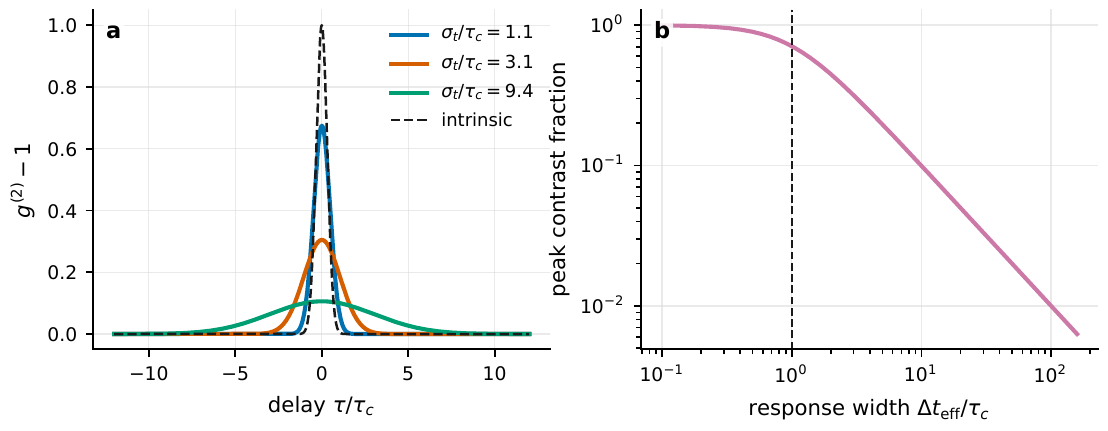
Figure 22 Finite timing response broadens and lowers a narrow thermal bunching peak. In the left panel, the dashed curve is the intrinsic picosecond-scale peak, while the solid curves show the observed peak after convolution with different response widths. The right panel shows that when \(\Delta t_{\rm eff}\gg\tau_c\), the zero-delay peak height falls roughly as \(\tau_c/\Delta t_{\rm eff}\).

The stellar bunching experiment of Guerin et al. gives useful numbers. The central wavelength was about \(7800\,\text{\AA}\), and the narrowest filter was \(10\,\text{\AA}\) wide, corresponding to \(\Delta\nu\simeq5\times10^{11}\,\mathrm{Hz}\) and \(\tau_c\simeq1.6\)–\(2\,\mathrm{ps}\). The single-photon timing jitter of the APDs was about \(500\,\mathrm{ps}\), and the relative response peak of the two detectors was about \(700\,\mathrm{ps}\) wide. For ideal thermal light \(C_{\rm true}=1\), but after convolution the expected observed peak was only \(C_{\rm obs}\simeq2.2\times10^{-3}\). The laboratory thermal source gave \((2.01\pm0.09)\times10^{-3}\), and the three bright stars gave peaks of about \(1.8\)–\(2.0\times10^{-3}\) [Guerin et al., 2017]. A telescope plot therefore does not usually show \(g^{(2)}(0)=2\). It may show \(1+10^{-3}\), \(1+10^{-6}\), or an even smaller excess.

The cross-correlation estimator in an event table can be written as a delay histogram. For two channels \(A\) and \(B\), delay-bin width \(\delta\tau\), and total live time \(T\),

(84)\[H_{AB}(\tau_m) = \sum_{i\in A}\sum_{j\in B} \mathbf{1}\!\left( \tau_m-\frac{\delta\tau}{2} \leq t_{B,j}-t_{A,i} < \tau_m+\frac{\delta\tau}{2} \right),\]

(85)\[\widehat g^{(2)}_{AB}(\tau_m) = \frac{H_{AB}(\tau_m)} {r_A r_B\,\delta\tau\,T}.\]

\(H_{AB}\) is a count. The denominator is also the expected number of accidental pairs, so \(\widehat g^{(2)}\) is dimensionless. Real analyses often avoid an analytic denominator and instead build a reference histogram \(H_{\rm ref}(\tau)\) from large time shifts, different observing segments, polarization-mismatched channels, or off-source data. The ratio or difference then absorbs unequal TDC bin widths, electronic crosstalk, slow transparency changes, and window-edge effects.

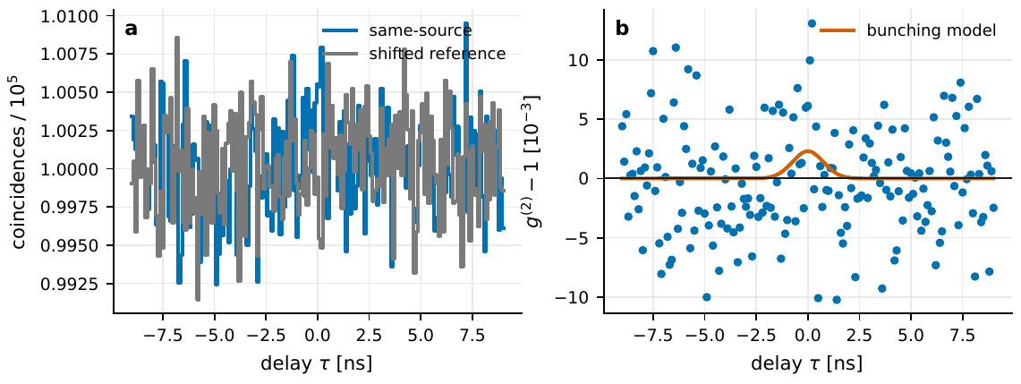
Figure 23 Structure of the delay-histogram estimator. In the left panel, event pairs from the source have a tiny excess near zero delay relative to the shifted reference histogram. In the right panel, the difference is normalized by the accidental-pair count to give g⁽²⁾ − 1, with a peak of order 10⁻³. Real observations must also correct for dead time, background, and the response function.

The dominant statistical error comes from the number of accidental pairs. If a delay bin contains \(N_{\rm pair}\) accidental coincidences, the shot-noise scale is

(86)\[\sigma\!\left[\widehat g^{(2)}(\tau)\right]\sim N_{\rm pair}^{-1/2}.\]

For two \(10^6\,\mathrm{s^{-1}}\) channels, \(\delta\tau=100\,\mathrm{ps}\), and \(T=1\,\mathrm{hr}\), the number of accidental pairs is about \(3.6\times10^8\), giving a single-bin statistical error of about \(5\times10^{-5}\). If the bunching peak spans several bins, one can fit the whole peak rather than use only the zero-delay bin. If system correlations sit at the \(10^{-3}\) level, better counting statistics will not help until TDC artifacts, electronic crosstalk, or background normalization are controlled. Guerin et al. approached the \(N^{-1/2}\) scaling after correcting TDC spurious correlations. Modern VERITAS and MAGIC systems extend the same idea to spatial intensity interferometry through offline correlation, GPU/FPGA correlators, and many-baseline averaging [Abeysekara et al., 2020, Abe et al., 2024, Guerin et al., 2017].

Higher-order, frequency-resolved, and polarization-resolved correlations

Second-order correlations use photon pairs. If three telescopes or three time channels are retained, one can define a third-order intensity correlation,

(87)\[g^{(3)}_{123}= \frac{\left\langle I_1 I_2 I_3\right\rangle} {\left\langle I_1\right\rangle \left\langle I_2\right\rangle \left\langle I_3\right\rangle}.\]

For Gaussian chaotic light, the third-order correlation contains second-order terms plus one closed-triangle term:

(88)\[g^{(3)}_{123} = 1 +|\gamma_{12}|^2+|\gamma_{23}|^2+|\gamma_{31}|^2 +2\,{\rm Re}\!\left(\gamma_{12}\gamma_{23}\gamma_{31}\right).\]

\(\gamma_{ij}\) is the first-order coherence between channels \(i\) and \(j\). The last term contains a closure phase. In principle, third-order intensity correlations can therefore recover part of the Fourier phase that is absent from second-order intensity interferometry. The cost is noise: photon triplets are much rarer than photon pairs and are more sensitive to systematics. Gamo’s early theory, the Ofir–Ribak approach, the imaging simulations of Nunez et al., and CTA-related studies all treat higher-order correlations as an important extension of intensity-interferometric imaging [Dravins and Lagadec, 2014, Dravins et al., 2013, Gamo, 1966, Nuñez et al., 2012, Nuñez et al., 2012].

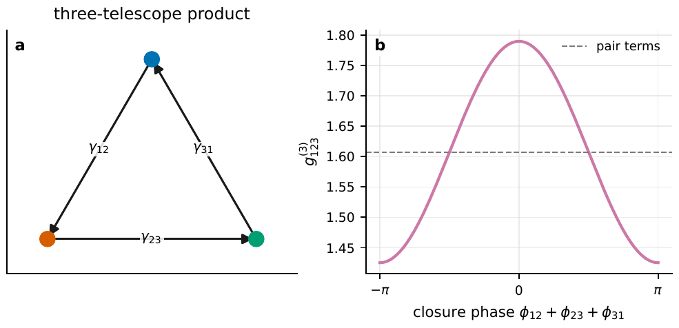
Figure 24 Origin of the closure-phase term in third-order intensity correlation. The left panel shows three telescopes forming the closed product γ₁₂γ₂₃γ₃₁. The right panel shows that, for fixed |γ_ij|, g⁽³⁾ varies with the cosine of the closure phase. Second-order intensity interferometry measures only |γ|²; the third-order term begins to carry phase-combination information.

Frequency- and polarization-resolved second-order correlations can be written as

(89)\[g^{(2)}_{pq}(\nu_1,\nu_2,\tau)= \frac{ \left\langle I_p(\nu_1,t)I_q(\nu_2,t+\tau)\right\rangle }{ \left\langle I_p(\nu_1,t)\right\rangle \left\langle I_q(\nu_2,t)\right\rangle } .\]

\(p,q\) are polarization channels, and \(\nu_1,\nu_2\) are frequencies or narrowband filter centers. If two frequency channels sample the same thermal line within its coherence width, their intensity fluctuations can be correlated. If they are separated by much more than the line width, the correlation should return to unity. If two polarizations come from the same physical emission process, cross-polarization correlations may probe magnetic or scattering geometry. If the polarization channels mix independent modes, the bunching peak is averaged down. For fast transients, pulsars, optical counterparts of FRBs, candidate astrophysical maser or laser lines, and extreme high-time-resolution observations, retaining event-level frequency and polarization labels is more valuable than storing only a total light curve [Foellmi, 2009, Nitu Rai et al., 2024, Tan et al., 2014].

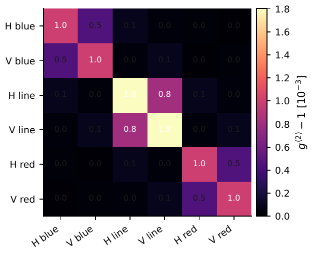
Figure 25 Frequency- and polarization-resolved g⁽²⁾ can be represented as a cross-channel matrix. Spectral-line channels have a larger excess because the coherence time is longer. Correlations within one polarization channel are often stronger than correlations between orthogonal polarization channels. Off-diagonal matrix elements measure common fluctuations across frequency and polarization.

In practice, the event table gives \(N\), \(H(\tau)\), and \(\widehat g^{(2)}\). Factorial moments and Mandel \(Q\) measure the width of the count distribution. The Siegert relation connects second-order intensity correlations of Gaussian thermal light to first-order coherence. Response convolution, mode number, and background fraction turn ideal optical-field quantities into \(10^{-3}\)–\(10^{-6}\) correlation peaks in real telescope data. Third-order, frequency-resolved, and polarization-resolved correlations bring phase combinations, line physics, and magnetic geometry into the same event-table language. Replacing time delay \(\tau\) with a spatial baseline \(\mathbf{B}\) takes the same correlation formalism into spatial coherence and intensity interferometry.