Mathematical and Physical Foundations

Chapter opening

A telescope does not receive an “image itself.” It receives a stream of photon events after the radiation has passed through the atmosphere, the optical system, filters, polarizers, detectors, and clocks. Accumulating those events into images, spectra, or light curves is the most common and most powerful form of data compression in astronomy. Quantum astronomy starts from the same events but keeps the arrival times, receiving locations, frequency channels, and polarization labels. It then asks about joint probabilities, coherence functions, and mode information. A minimal event row gives the language of the data. Phase, spatial coherence, counting statistics, intensity correlations, polarization, quantum states, and likelihood functions give the physical language for interpreting those data. These tools come from statistical optics, quantum optics, Fourier optics, interferometry, and quantum estimation theory. In observations, however, they eventually have to return to photon rates, coherence times, baselines, backgrounds, and error budgets [Glauber, 1963, Glauber, 1963, Goodman, 2000, Goodman, 2005, Mandel and Wolf, 1965, Mandel and Wolf, 1995, Wolf, 2007].

From Event Tables to Observables

A single photon detection may be written as

(1)\[e_j=(t_j,\bm{r}_j,\nu_j,p_j,w_j).\]

Here \(t_j\) is the time stamp of the \(j\)-th event, usually measured in seconds, nanoseconds, or picoseconds. The vector \(\bm{r}_j\) denotes the telescope, detector pixel, or array position that received the event, with lengths measured in meters. The quantity \(\nu_j\) is the frequency channel in Hz. The label \(p_j\) denotes polarization, for example horizontal, vertical, left circular, or right circular. The weight \(w_j\) may encode an efficiency correction, a background estimate, a quality cut, or a bad-pixel mask. Real data products also contain energy, detector identifiers, trigger quality, dead-time flags, and weather information, but Eq. (1) is the minimal structure needed in this book.

Images, spectra, and light curves are projections of an event table. Binning events by sky position gives \(I(x,y)\); binning them by frequency gives \(I(\nu)\); binning them by time gives \(I(t)\). These products answer first-order questions: what the mean brightness is, what the spectral energy distribution is, and how the source varies in time. If event pairs or event groups are retained, one can estimate second- and higher-order statistics, such as coincidence counts between two telescopes in the same time window, covariances between frequency channels, or correlations between polarization channels. Glauber’s theory of optical coherence writes these observables as correlation functions of field operators, while the statistical-optics framework of Mandel, Wolf, and Goodman gives the standard route from electromagnetic fields and coherence functions to photodetection [Glauber, 1963, Glauber, 1963, Goodman, 2000, Mandel and Wolf, 1965, Mandel and Wolf, 1995].

The first meaning of an event table is counting. Once interferometry enters the problem, direction of arrival, optical path difference, and wavelength together set a phase. A single detector usually preserves only intensity. When two beams are superposed, the electric fields add first and the intensity is formed afterward; the phase difference can then become a measurable fringe, a visibility, or a correlation of intensity fluctuations.

Complex Amplitude, Phase, and Interference

Within a sufficiently narrow frequency channel, an electromagnetic wave can be approximated as monochromatic. The physical electric field \(E(t)\) is real, but amplitude and phase are easier to track with a complex notation. Define the complex amplitude

(2)\[\mathcal{E}=E_0 e^{i\phi}, \qquad E(t)=\operatorname{Re}\!\left[\mathcal{E}e^{i\omega t}\right].\]

The number \(\mathcal{E}\) is the complex amplitude. Its modulus \(E_0=|\mathcal{E}|\) gives the field scale, and its argument \(\arg\mathcal{E}=\phi\) gives the phase of the beam at the point of interest. The angular frequency is \(\omega=2\pi\nu\), with units \(\mathrm{rad\,s^{-1}}\); \(\nu\) is the ordinary frequency; and \(\phi\) is measured in radians. If \(\mathcal{E}\) represents the physical electric-field amplitude, it may be given in \(\mathrm{V\,m^{-1}}\), like \(E(t)\). If it represents a quantum-optical mode amplitude, the single-photon energy and mode normalization are often absorbed into the mode function, leaving the amplitude dimensionless. Optical frequencies are roughly \(4\times10^{14}\) to \(8\times10^{14}\,\mathrm{Hz}\), so one optical cycle lasts only a few femtoseconds. Ordinary astronomical detectors do not record \(E(t)\) cycle by cycle. They record energy, photon counts, or coincidences averaged over many optical cycles. Phase is therefore not read directly from an electric-field trace; it enters the data through interference, correlations, or mode projection.

When two beams enter the same detector, the fields add before the intensity is formed:

(3)\[I \propto |\mathcal{E}_1+\mathcal{E}_2|^2 = |\mathcal{E}_1|^2+|\mathcal{E}_2|^2 +2\,\operatorname{Re}(\mathcal{E}_1\mathcal{E}_2^\ast).\]

If \(\mathcal{E}_1=E_1e^{i\phi_1}\) and \(\mathcal{E}_2=E_2e^{i\phi_2}\), with \(E_1,E_2\ge0\), the interference term is \(2E_1E_2\cos(\phi_1-\phi_2)\). The first two terms are the separate beam intensities; the third term is the measurable trace of the phase difference. Constructive interference corresponds to \(\phi_1-\phi_2\simeq0\), and destructive interference to \(\phi_1-\phi_2\simeq\pi\). If optical-path disturbances make the phase difference sweep through many radians during an exposure, the interference term averages away and only the summed intensities remain.

Amplitude interferometers preserve first-order phase information. The complex fields received by two telescopes must be combined coherently on wavelength scales, so the optical path difference has to be controlled to much less than \(\lambda\). At \(\lambda=500\,\mathrm{nm}\), half a wavelength is only \(250\,\mathrm{nm}\); atmospheric turbulence, mechanical vibration, and thermal expansion are all large enough to move the phase. Intensity interferometry does not combine electric fields directly. It compares intensity fluctuations at two telescopes. It loses the phase of the complex visibility, but retains the squared visibility amplitude \(|V|^2\). The Hanbury Brown and Twiss experiments used precisely this correlation of intensity fluctuations to establish photon correlation measurements and stellar intensity interferometry [Brown and Twiss, 1956, Brown and Twiss, 1957, Hanbury Brown, 1956, Hanbury Brown, 1974].

The phase most often encountered in astronomy is the dimensionless quantity \(2\pi\bm{b}\cdot{\boldsymbol s}/\lambda\), where \(\bm{b}\) is the baseline vector, \({\boldsymbol s}\) is the unit vector toward the source, and \(\lambda\) is the wavelength. Baseline, direction, and wavelength determine the phase geometrically; the detector and data analysis determine whether that phase can still be estimated.

Fourier Visibility and Sky Brightness

Let the sky brightness distribution be \(I(l,m)\). The variables \(l\) and \(m\) are small angular direction cosines relative to the phase center, and may be treated as radians in a narrow field. The function \(I(l,m)\) is the brightness per unit solid angle and per unit frequency or wavelength. Dividing the projected baseline between two telescopes by the wavelength gives the dimensionless spatial frequencies

(4)\[u=\frac{B_x}{\lambda},\qquad v=\frac{B_y}{\lambda}.\]

Here \(B_x\) and \(B_y\) are the projected baseline components in the two directions of the tangent plane, in meters, and \(\lambda\) is the observing wavelength. If the baseline length is of order \(B\), then the spatial frequency is of order \(u\sim B/\lambda\). At visible wavelengths, \(\lambda=500\,\mathrm{nm}\) and \(B=100\,\mathrm{m}\) give \(u\sim2\times10^8\).

The normalized complex visibility is

(5)\[V(u,v)= \frac{\int I(l,m)e^{-2\pi i(ul+vm)}\,dl\,dm} {\int I(l,m)\,dl\,dm}.\]

The denominator is the total flux, so \(V(0,0)=1\). The exponential factor is the phase fringe laid across the sky by the baseline. A baseline does not measure an image. It measures a weighted integral of the sky brightness against a pattern of alternating positive and negative fringes. Zernike’s and van Cittert’s coherence concepts, Fourier optics, and modern interferometry all write this measurement as sampling in the \(u,v\) plane [Goodman, 2005, van Cittert, 1939, Wolf, 2007, Zernike, 1938].

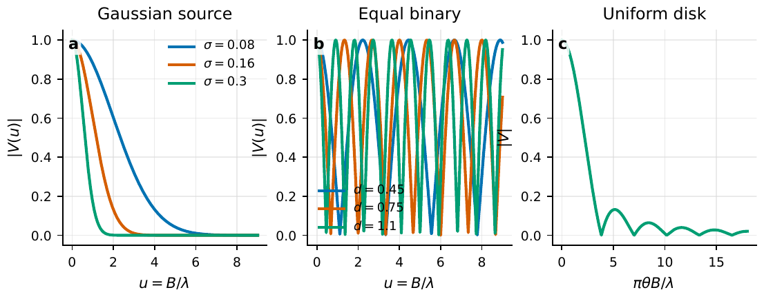
Figure 1 Normalized visibility curves for a Gaussian source, an equal-brightness binary, and a uniform disk. Larger angular scales make the visibility fall faster with spatial frequency; binaries produce visibility oscillations; uniform disks have zeros and sidelobes because their edges are sharper.

The three source classes in Fig. Figure 1 will recur throughout the book. A point source has no angular structure and ideally gives \(|V|=1\) on every baseline. A Gaussian source of width \(\sigma_\theta\) remains a Gaussian in Fourier space, with a characteristic falloff at spatial frequency of order \(1/\sigma_\theta\). A binary can be approximated by two point sources; if their angular separation is \(\Delta\theta\), the visibility oscillates with \(u\Delta\theta\). The oscillation period gives the separation, while the amplitude depends on the flux ratio. A thin ring or photon ring also produces oscillations, but with a different envelope and different zero locations. That picture will be used later when black-hole photon rings are discussed.

For a uniform disk, the analytic visibility model is

(6)\[V(x)=\frac{2J_1(x)}{x},\qquad x=\frac{\pi B\theta}{\lambda}.\]

Here \(J_1\) is the first-order Bessel function. The quantity \(B\) is the projected baseline length in meters, \(\theta\) is the disk angular diameter in radians, \(\lambda\) is the wavelength, and \(x\) is dimensionless. It measures how strongly the disk is resolved by the baseline. When \(x\ll1\), the disk is nearly unresolved and \(|V|\simeq1-x^2/8\). When \(x\) reaches the first zero of \(J_1\), at \(3.8317\), the visibility first vanishes. Intensity interferometry measures \(|V|^2\), so the zeros and sidelobes remain useful, although the complex phase is not directly retained. The Narrabri intensity interferometer measured stellar angular diameters with this family of disk and limb-darkened models [Hanbury Brown, 1974, Hanbury Brown et al., 1967, Hanbury Brown et al., 1967].

A first estimate of angular resolution is

(7)\[\theta_{\rm res}\sim \frac{\lambda}{B}.\]

The angular scale \(\theta_{\rm res}\) is in radians. With \(\lambda=500\,\mathrm{nm}\) and \(B=100\,\mathrm{m}\), one obtains \(\theta_{\rm res}\sim5\times10^{-9}\,\mathrm{rad}\), about \(1\,\mathrm{mas}\). A target structure of \(10\,\mu\mathrm{as}\) at the same wavelength requires baselines of order \(10\,\mathrm{km}\). This estimate only tests whether the baseline reaches the target angular scale. It does not replace an error budget. Parameter errors also depend on photon rate, background, baseline coverage, bandwidth, time resolution, and model degeneracies.

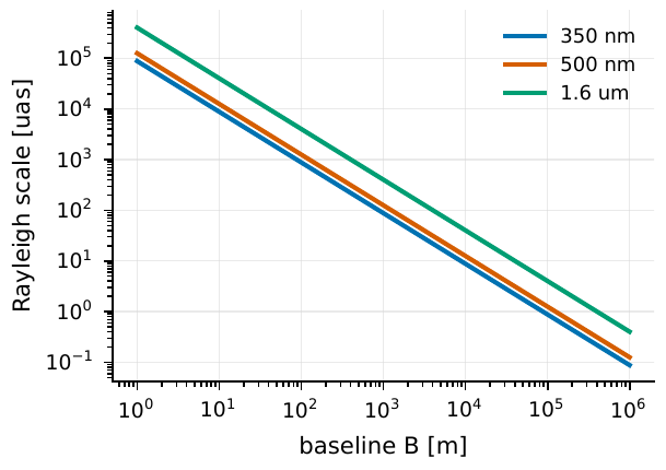
Figure 2 Angular-resolution scale as a function of wavelength and baseline. At visible wavelengths, milliarcsecond scales require baselines of order one hundred meters, while ten-microarcsecond scales require kilometer to ten-kilometer baselines.

Ground-based arrays must also consider \(u,v\) coverage. The same physical baseline traces a track in the \(u,v\) plane as Earth rotates. Multiple telescopes provide multiple tracks; weather, target elevation, and array geometry leave gaps. Amplitude-interferometric imaging needs enough complex visibility samples to reconstruct the brightness distribution. Intensity interferometry measures only \(|V|^2\). Without closure phase, image reconstruction is harder, but parameterized models remain powerful. Stellar diameters, binary separations, limb-darkening coefficients, and ring radii can all be estimated from the shape of \(|V|^2(B/\lambda)\).

Photon Counting Distributions and Factorial Moments

Choose a time bin of width \(\Delta t\), and count \(N\) photons in that bin. If the photon arrival rate is \(R_\gamma\), the mean count is

(8)\[\mu=R_\gamma\Delta t.\]

The rate \(R_\gamma\) has units \(\mathrm{s^{-1}}\), \(\Delta t\) is measured in seconds, and \(\mu\) is a dimensionless mean photon count. In an event table, \(N\) is the number of events with \(t_j\in[t,t+\Delta t)\) that pass the quality cuts. If the events are also filtered by telescope, frequency, or polarization, then \(R_\gamma\) and \(\mu\) refer to that selected channel.

Independently arriving photons follow a Poisson distribution:

(9)\[P(N)=e^{-\mu}\frac{\mu^N}{N!},\qquad \operatorname{Var}(N)=\mu.\]

Here \(P(N)\) is the probability of counting \(N\) photons, and \(\operatorname{Var}(N)\) is the count variance. The Poisson standard deviation is \(\sqrt{\mu}\), so the relative shot noise is \(1/\sqrt{\mu}\). At \(\mu=10^4\), the relative fluctuation is about \(1\%\). At \(\mu=1\), the discreteness of the counts is itself the dominant noise. A coherent state has Poisson counting statistics; in quantum optics it is the idealized light field closest to a classical stable wave.

The photon-count distribution of single-mode thermal light is the Bose–Einstein distribution,

(10)\[P(N)=\frac{\bar n^N}{(1+\bar n)^{N+1}}.\]

The mean photon occupation of the mode is \(\bar n=\langle N\rangle\). This distribution is broader than a Poisson distribution, with variance \(\bar n(1+\bar n)\). The extra width comes from intensity fluctuations, or photon bunching. At zero delay, single-mode thermal light satisfies

(11)\[g^{(2)}(0)= \frac{\langle N(N-1)\rangle}{\langle N\rangle^2}=2.\]

The quantity \(\langle N(N-1)\rangle\) is a second factorial moment. Coincidence counting naturally uses \(N(N-1)\), because \(N\) photons in a bin form \(N(N-1)\) ordered photon pairs. The ordinary \(N^2\) would also count a photon paired with itself. Glauber’s coherence theory generalizes these factorial moments to normally ordered field correlation functions [Glauber, 1963, Mandel and Wolf, 1995].

The bunching contrast of multimode thermal light is diluted. If the effective number of independent modes in one time-frequency-polarization-spatial cell is \(M\), a common approximation is

(12)\[g^{(2)}(0)=1+\frac{1}{M}.\]

For \(M=1\), this reduces to the single-mode thermal value \(g^{(2)}(0)=2\). For \(M\gg1\), the excess \(g^{(2)}(0)-1\) becomes small. Astronomical observations easily enter the multimode regime: broadband filters, long time bins, finite angular apertures, multiple polarizations, and multiple spatial modes all increase \(M\). As a result, the large bunching peak seen in laboratory thermal light often becomes a weak excess correlation of \(10^{-6}\) to \(10^{-2}\) in telescope data.

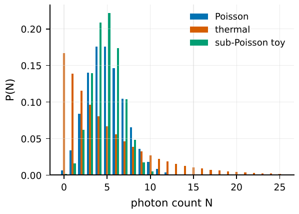
Figure 3 Poisson, single-mode thermal, and sub-Poisson toy distributions with the same mean photon count. The width of the distribution determines the Mandel Q parameter and the direction in which the second-order coherence departs from 1.

The Mandel \(Q\) parameter writes the width of a count distribution as

(13)\[Q=\frac{\operatorname{Var}(N)-\langle N\rangle}{\langle N\rangle}.\]

Poisson statistics give \(Q=0\). Super-Poisson statistics have \(Q>0\); thermal light belongs to this class. Sub-Poisson statistics have \(Q<0\), which is uncommon for astronomical thermal radiation but appears in quantum-optics experiments with single atoms or controlled light sources. Mandel’s sub-Poisson statistics and the antibunching experiment of Kimble, Dagenais, and Mandel showed that \(g^{(2)}<1\) is an important signature of nonclassical light [Kimble et al., 1977, Mandel, 1979]. If an astronomical data set appears to show \(g^{(2)}<1\) or \(Q<0\), the first step is to check dead time, pile-up, threshold selection, background subtraction, and multiple testing, not to announce a nonclassical astrophysical light source.

Covariance, HBT Correlations, and Noise

Let \(N_1\) and \(N_2\) be the counts recorded by two telescopes in the same time bin. If the two streams are merely independent fluctuations, a high value of \(N_1\) does not imply a high value of \(N_2\). If they sample the same thermal light field at two spatial locations, their intensity fluctuations have a weak common component. The covariance is

(14)\[\operatorname{Cov}(N_1,N_2) =\langle N_1N_2\rangle-\langle N_1\rangle\langle N_2\rangle.\]

Angle brackets denote an average over many time bins, short exposures, or statistically equivalent samples. The first term is the mean product of the observed coincidences; the second is the expected accidental coincidence level. Their difference contains physical correlations, background correlations, instrumental crosstalk, and residual systematics. Later analyses must separate these contributions.

The normalized second-order correlation function may be written as

(15)\[g^{(2)}_{12}(\tau)= \frac{\langle N_1(t)N_2(t+\tau)\rangle} {\langle N_1(t)\rangle\langle N_2(t+\tau)\rangle}.\]

The delay \(\tau\) is measured in seconds. In an event table, this quantity can be estimated with a delay histogram: for each event in telescope 1, find events in telescope 2 whose time differences fall in \([\tau,\tau+\Delta\tau)\), then divide by the accidental coincidence count predicted by the single-channel rates. If \(g^{(2)}_{12}=1\), there is no measurable excess correlation. If \(g^{(2)}_{12}>1\), the two channels are positively correlated. For ideal chaotic light, and assuming a narrow band, stationarity, linear detectors, and negligible background, the Siegert relation gives

(16)\[g^{(2)}_{12}(0)-1 \simeq |\gamma^{(1)}_{12}|^2.\]

The quantity \(\gamma^{(1)}_{12}\) is the normalized first-order coherence between the two telescopes, equivalent to the corresponding sample of the normalized complex visibility \(V\). Intensity interferometry measures \(|\gamma^{(1)}|^2\). It can therefore measure angular scales and some geometric parameters, but it does not by itself provide the complex phase. The original HBT papers, the Sirius intensity-interferometer test, the correlation theory papers, and the later Narrabri observations took this relation from the laboratory to stellar angular-diameter measurements [Brown and Twiss, 1956, Brown and Twiss, 1957, Brown and Twiss, 1958, Hanbury Brown, 1956, Hanbury Brown et al., 1967].

Real observations must also include dilution by finite time resolution. The field coherence time satisfies the order-of-magnitude relation

(17)\[\tau_c\sim\frac{1}{\Delta\nu}.\]

Here \(\Delta\nu\) is the frequency bandwidth in Hz, and \(\tau_c\) is the coherence time in seconds. If the detector response or analysis bin width \(\Delta t\gg\tau_c\), the bunching peak is averaged down, and the observed excess correlation is reduced roughly by \(\tau_c/\Delta t\):

(18)\[g^{(2)}_{\rm obs}(0)-1 \simeq |\gamma^{(1)}_{12}|^2\frac{\tau_c}{\Delta t}.\]

This expression assumes rectangular time bins, a stationary light field, and \(\Delta t\) much larger than the coherence time. In a real instrument, \(\tau_c/\Delta t\) should be replaced by the convolution of the spectral and temporal response functions. Near \(\lambda=500\,\mathrm{nm}\), a \(1\,\mathrm{nm}\) optical band corresponds to \(\Delta\nu\sim10^{12}\,\mathrm{Hz}\), or \(\tau_c\sim1\,\mathrm{ps}\). If the time bin is \(100\,\mathrm{ps}\), the contrast is reduced by about \(10^{-2}\). If the electronic response is \(1\,\mathrm{ns}\), only a \(10^{-3}\)-level contrast remains. The zero-baseline amplitudes in full stellar photon-bunching experiments and in VERITAS/MAGIC system papers fall near these scales [Abeysekara et al., 2020, Abe et al., 2024, Guerin et al., 2017].

Background and detector effects change the normalization. If the source count rate is \(S\), the background count rate is \(B\), and the background is uncorrelated with the source, the source correlation is diluted to

(19)\[g^{(2)}_{\rm meas}-1 \simeq (g^{(2)}_{\rm src}-1) \left(\frac{S}{S+B}\right)^2.\]

Both \(S\) and \(B\) have units \(\mathrm{s^{-1}}\). When sky background, dark counts, or neighboring sources contribute count rates comparable to the target, the correlation signal falls quadratically. Dead time suppresses short-delay coincidences, afterpulsing creates false positive correlations, and clock drift broadens or shifts the correlation peak. Null tests in HBT analyses usually include swapping time segments, using delay windows far from the physical delay, comparing non-adjacent frequency channels, scrambling event times, and checking dark-field data.

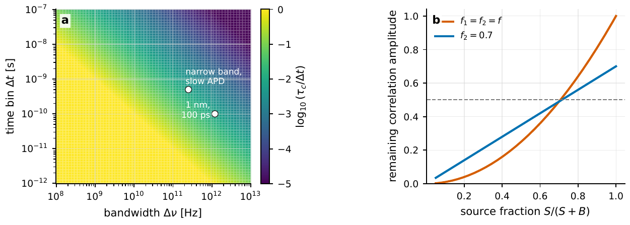
Figure 4 The scale of an HBT correlation peak is set jointly by time-resolution dilution and background dilution. The left panel shows τ_c/Δt as a function of optical bandwidth and time-bin width, with white points marking common narrow-band optical observing regimes. The right panel shows how the correlation amplitude is lost as f₁f₂ when the source-photon fractions in the two channels decrease.

Multi-channel observations generalize covariance to a matrix,

(20)\[C_{ab}=\langle (N_a-\bar N_a)(N_b-\bar N_b)\rangle.\]

The indices \(a,b\) may label telescopes, frequencies, polarizations, time windows, or spatial modes. The diagonal entries of \(C_{ab}\) are the variances of individual channels; the off-diagonal entries are shared fluctuations between channels. When later chapters discuss spectral correlations, polarization correlations, array baselines, and quantum-network telescopes, the likelihood often contains such a covariance matrix rather than a single \(g^{(2)}\).

Matrices, Polarization, and Instrument Response

An electromagnetic wave propagating along the line of sight has two transverse polarization degrees of freedom. The Jones vector is

(21)\[\begin{split}\bm{E}= \begin{pmatrix} E_x\\ E_y \end{pmatrix},\end{split}\]

where \(E_x\) and \(E_y\) are the complex amplitudes in two orthogonal polarization directions. In the approximation of fully coherent and fully polarized light, an ideal linear polarizer, retarder, mirror, or fiber coupler can be represented by a Jones matrix,

(22)\[\bm{E}_{\rm out}=J\bm{E}_{\rm in}.\]

The matrix \(J\) is a \(2\times2\) complex matrix. Its diagonal entries describe transmission and phase delay in the same polarization; its off-diagonal entries describe polarization mixing. Jones notation is well suited to describing how optical elements act on complex electric fields, but most astronomical detectors measure intensities and do not directly measure the complex phases of \(E_x\) and \(E_y\).

Astronomical polarimetry usually uses the Stokes vector,

(23)\[\bm{S}=(I,Q,U,V)^{\mathsf T}.\]

Here \(I\) is total intensity; \(Q\) is the intensity difference between horizontal and vertical linear polarization; \(U\) is the intensity difference between \(+45^\circ\) and \(-45^\circ\) linear polarization; and \(V\) is the intensity difference between right- and left-circular polarization. If the efficiencies of four measurement channels have been calibrated, one may use

(24)\[Q=I_H-I_V,\qquad U=I_{45}-I_{135},\qquad V=I_R-I_L.\]

These quantities have the same intensity units as \(I\). The degree of linear polarization and the polarization angle are often written as

(25)\[p_L=\frac{\sqrt{Q^2+U^2}}{I},\qquad \chi=\frac{1}{2}\arctan\!\frac{U}{Q}.\]

The degree \(p_L\) is dimensionless, and \(\chi\) is measured in radians or degrees. Many astronomical sources have optical linear polarization between \(10^{-3}\) and \(10^{-1}\). Synchrotron jets or environments with highly ordered magnetic fields can be more strongly polarized. Interstellar dust, telescope reflections, and detector response can produce signals of comparable size. Standard astronomical polarization notation and calibration procedures are reviewed by Tinbergen [1996].

The action of an instrument on a Stokes vector is described by a Mueller matrix,

(26)\[\bm{S}_{\rm obs}=M\bm{S}_{\rm sky}.\]

The vector \(\bm{S}_{\rm sky}\) is the incident Stokes vector from the source, \(\bm{S}_{\rm obs}\) is the estimated instrumental output, and \(M\) is a \(4\times4\) real matrix. Diagonal terms give transmission and efficiency for the Stokes components; off-diagonal terms give crosstalk. For example, \(M_{21}\) leaks total intensity \(I\) into \(Q\), while \(M_{23}\) makes true \(U\) appear as \(Q\). If a target polarization angle rotates by only \(0.1^\circ\), and the off-diagonal Mueller elements are calibrated only to \(10^{-3}\), the systematic error is already on the same scale as the signal. Instrumental polarization can arise from reflections, obscuration, and off-axis optical paths in the telescope focal plane. It cannot be ignored in searches for strong-field QED, cosmic birefringence, or axion-induced polarization effects [Rubin et al., 2019, Sanchez Almeida and Martinez Pillet, 1992].

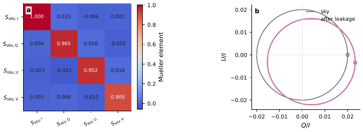
Figure 5 Effect of Mueller-matrix crosstalk on a weak polarization signal. The left panel shows an example instrument matrix with percent-level transmission errors and 10⁻³–10⁻²-level crosstalk. The right panel shows how a true 2% linear-polarization track in the Q − U plane is shifted and stretched by I → Q leakage and Q ↔︎ U crosstalk.

Stokes vectors and Mueller matrices describe mean polarization signals. If an event table keeps polarization labels, the same labels can also enter second-order statistics. Separating events into \(H,V,R,L\) and similar channels, one may define

(27)\[g^{(2)}_{pq}(\tau)= \frac{\langle N_p(t)N_q(t+\tau)\rangle} {\langle N_p(t)\rangle\langle N_q(t+\tau)\rangle},\]

where \(p,q\) denote polarization channels. Unpolarized thermal light may be treated as two independent orthogonal polarization modes. Same-polarization channels preserve thermal bunching, while excess correlations in orthogonal cross-polarization channels are weakened or vanish. If the radiation mechanism, magnetic field, or propagation effect selects a particular polarization, \(g^{(2)}_{HH}\), \(g^{(2)}_{HV}\), and \(g^{(2)}_{RR}\) can differ. In real data, that difference is always superposed on polarization efficiency, crosstalk, and channel-to-channel timing calibration.

States, Density Matrices, and Photodetection

Quantum notation describes optical states and detection operators. If the system is in a pure state \(|\psi\rangle\), the expectation value of an observable \(\hat O\) is

(28)\[\langle \hat O\rangle=\langle\psi|\hat O|\psi\rangle.\]

Here \(|\psi\rangle\) is the state vector, \(\langle\psi|\) is its conjugate transpose, and \(\hat O\) may be a photon-number operator, a mode-projection operator, or a field-correlation operator. Stable laboratory lasers are often well approximated as coherent states. Single-photon sources, squeezed light, and entangled light require a fuller quantum-state description. Astrophysical thermal radiation, accretion-disk emission, scattered light, and light that has passed through loss are usually not pure states.

Mixed states are represented by a density matrix \(\rho\):

(29)\[\langle \hat O\rangle=\operatorname{Tr}(\rho\hat O),\]

where \(\rho\) is a density operator with \(\operatorname{Tr}\rho=1\), and \(\operatorname{Tr}\) denotes a trace over diagonal elements. A single-mode thermal state can be written in the photon-number basis as

(30)\[\rho_{\rm th}=\sum_{n=0}^{\infty} \frac{\bar n^n}{(1+\bar n)^{n+1}}\,|n\rangle\langle n|.\]

Here \(|n\rangle\) is an \(n\)-photon Fock state, and \(\bar n\) is the mean occupation number. This density matrix is diagonal, meaning that the phase has been randomized. It gives exactly the photon-number probabilities in Eq. (10).

Unrecorded degrees of freedom do not disappear from the physical system, but they cannot be used as distinguishable information in the data. If the full system consists of the observed modes \(A\) and unobserved modes \(B\), the observer must sum over all possible states of \(B\), obtaining the state available for data analysis:

(31)\[\rho_A=\operatorname{Tr}_B(\rho_{AB}).\]

The operation \(\operatorname{Tr}_B\) is a partial trace over the degrees of freedom in \(B\); it averages over whatever was not recorded. Here \(B\) may be an unrecorded frequency, polarization, spatial mode, time mode, environmental scattering degree of freedom, or detector-loss channel. This operation explains why lost modes reduce coherence, and why broadband, multimode, long-bin astronomical thermal light is better described as a mixed state.

The ideal photodetection rate is proportional to a field correlation, but the operator ordering follows the absorption process: creation operators appear on the left and annihilation operators on the right. This is normal ordering. A single-photon count rate may be written as

(32)\[R(t)\propto \langle \hat E^{(-)}(t)\hat E^{(+)}(t)\rangle.\]

The operator \(\hat E^{(+)}\) is the positive-frequency electric field, associated with photon annihilation, and \(\hat E^{(-)}\) is its Hermitian conjugate, associated with photon creation. Second-order coincidence counting involves

(33)\[G^{(2)}(1,2)= \left\langle \hat E_1^{(-)}\hat E_2^{(-)} \hat E_2^{(+)}\hat E_1^{(+)} \right\rangle.\]

The labels 1 and 2 may denote two times, two telescopes, two frequency channels, or two polarization channels. Equation (33) is the quantum version of Eq. (15): detectors record photon events, and the correlation function records the probability that events occur together. Normal ordering ensures that vacuum fluctuations are not counted as real clicks by an ideal direct photon counter.

Likelihood Functions and Fisher Information

Suppose event arrivals follow an inhomogeneous Poisson process, and the model predicts a time-dependent rate \(r(t;\boldsymbol{\theta})\). The rate \(r\) has units \(\mathrm{s^{-1}}\), and \(\boldsymbol{\theta}\) is a parameter vector, for example angular diameter, binary separation, background rate, coherence time, polarization angle, or instrumental delay. If events \(t_1,\ldots,t_n\) are recorded in the observing window \([T_0,T_1]\), the unbinned event-table log-likelihood is

(34)\[\ln L(\boldsymbol{\theta}) =\sum_{j=1}^{n}\ln r(t_j;\boldsymbol{\theta}) -\int_{T_0}^{T_1} r(t;\boldsymbol{\theta})\,dt.\]

The first term evaluates the model rate at the actual event times. The second term is the total number of events predicted by the model. If the data are divided into bins, with model mean \(\mu_k(\boldsymbol{\theta})\) and observed count \(N_k\) in bin \(k\), then

(35)\[\ln L=\sum_k \left[ N_k\ln\mu_k-\mu_k-\ln(N_k!) \right].\]

Only when the count in each bin is large and the errors are approximately Gaussian does Eq. (35) reduce to the familiar \(\chi^2\) fit. Low counts, fast transients, coincidence counts, and event-time analyses are better handled with the Poisson likelihood directly. The Cash statistic used in X-ray and high-energy astronomy comes from this Poisson likelihood. Modern MCMC or nested-sampling algorithms merely search the parameter space outside the likelihood; they do not replace the physical modeling of event rates, backgrounds, and selection functions [Cash, 1979, Feroz et al., 2009, Foreman-Mackey et al., 2013].

Fisher information measures the sensitivity of the data distribution to changes in model parameters:

(36)\[F_{\alpha\beta} =\left\langle \frac{\partial\ln L}{\partial\theta_\alpha} \frac{\partial\ln L}{\partial\theta_\beta} \right\rangle.\]

The quantities \(\theta_\alpha\) and \(\theta_\beta\) are parameter components, and \(F_{\alpha\beta}\) is an element of the Fisher matrix. For independent Poisson bins,

(37)\[F_{\alpha\beta} =\sum_k \frac{1}{\mu_k} \frac{\partial\mu_k}{\partial\theta_\alpha} \frac{\partial\mu_k}{\partial\theta_\beta}.\]

In this form, the constraining power comes from \(\partial\mu_k/\partial\theta_\alpha\), not from the count itself. If the model count \(\mu_k\) in a bin is insensitive to the parameter, that bin contributes little Fisher information. If background makes \(\mu_k\) large but the derivative is dominated by background rather than by the target, the target parameter is not measured more precisely.

The Cramer–Rao bound is

(38)\[\operatorname{Var}(\hat\theta_\alpha)\ge (F^{-1})_{\alpha\alpha}.\]

Here \(\hat\theta_\alpha\) is an unbiased estimator, and \(\operatorname{Var}\) is the estimator variance. Two observing designs may have the same \(\lambda/B\) but very different Fisher matrices because they have different photon counts, backgrounds, baseline distributions, frequency coverage, and mode measurements. Helstrom’s quantum detection and estimation theory, and the Braunstein–Caves quantum statistical distance, extend this idea to the limits set by the quantum measurement itself [Braunstein and Caves, 1994, Helstrom, 1969].

Quantum Fisher information gives the best achievable precision over all allowed measurements. If a measurement reaches the quantum-Fisher bound, no other detection strategy can do better with the same photon number and the same state. Weak-thermal-light superresolution theory shows that direct imaging can discard a large amount of Fisher information in the small-separation limit, whereas spatial-mode decomposition can recover it [Tsang, 2015, Tsang et al., 2016]. Later, in the discussion of quantum-network telescopes, quantum Fisher information will be used to compare local detection, entanglement-assisted measurements, and quantum-memory schemes.

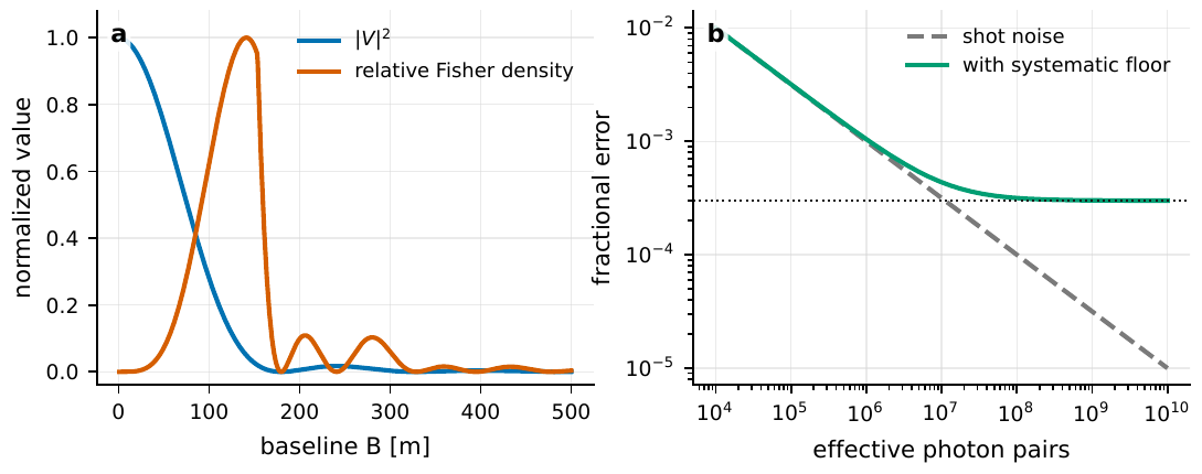
Figure 6 Fisher information turns the question “is the baseline long enough?” into “does the slope of the visibility curve, together with the measurement error, carry information about the parameter?” The left panel uses a 0.7 mas uniform disk; the steep part of the |V|² curve contributes most angular-diameter information. The right panel shows the statistical error falling with the number of effective photon pairs until a systematic floor stops further improvement.

Order-of-Magnitude Toolkit

Time resolution and optical path difference are related by

(39)\[\Delta \ell=c\,\Delta t.\]

Here \(c\simeq3.0\times10^8\,\mathrm{m\,s^{-1}}\) is the speed of light, \(\Delta t\) is the timing error, and \(\Delta\ell\) is the corresponding path error. A timing error of \(1\,\mathrm{ps}\) corresponds to about \(0.3\,\mathrm{mm}\), and \(1\,\mathrm{ns}\) to about \(0.3\,\mathrm{m}\). Intensity interferometry can tolerate larger path errors than amplitude interferometry, but time synchronization still determines whether the correlation peak is broadened or shifted.

A practical conversion between wavelength bandwidth and coherence time comes from

(40)\[\Delta\nu\simeq \frac{c\,\Delta\lambda}{\lambda^2}.\]

Here \(\Delta\lambda\) is the wavelength bandwidth. For \(\lambda=500\,\mathrm{nm}\) and \(\Delta\lambda=1\,\mathrm{nm}\), one finds \(\Delta\nu\simeq1.2\times10^{12}\,\mathrm{Hz}\), so \(\tau_c\sim1/\Delta\nu\) is of order a picosecond. A \(0.01\,\mathrm{nm}\) narrow band can increase \(\tau_c\) to hundreds of picoseconds, but the photon rate decreases approximately linearly with the bandwidth.

The photon rate can be estimated from the spectral flux:

(41)\[R_\gamma=A\eta\int F_\lambda\frac{\lambda}{hc}\,d\lambda.\]

Here \(R_\gamma\) is the detected photon rate in \(\mathrm{s^{-1}}\), \(A\) is the effective collecting area in \(\mathrm{m^2}\), and \(\eta\) is the total efficiency, including atmosphere, optical transmission, filters, and detector quantum efficiency. Typical \(\eta\) values range from \(0.01\) to \(0.5\). The spectral flux density is \(F_\lambda\), and the factor \(\lambda/(hc)\) converts energy flux into photon-number flux. In the AB magnitude system one may also write

(42)\[F_\nu=3631\,\mathrm{Jy}\,10^{-0.4m_{\rm AB}}, \qquad R_\gamma\simeq A\eta\,\frac{F_\nu\Delta\nu}{h\nu}.\]

Every increase of 5 magnitudes in \(m_{\rm AB}\) decreases the flux by a factor of 100. Telescope area and efficiency increase the photon rate only linearly, so target brightness is usually the first constraint in a feasibility estimate.

Quantity	Typical range	Physical meaning
\(\lambda\)	\(350\,\mathrm{nm}\) to \(1.6\,\mu\mathrm{m}\)	Observing wavelength; shorter wavelengths give higher angular resolution at fixed baseline.
\(B\)	\(10\,\mathrm{m}\) to \(10\,\mathrm{km}\)	Projected baseline; sets the spatial frequency \(u\sim B/\lambda\).
\(\theta\)	\(10\,\mu\mathrm{as}\) to several mas	Typical scales for stellar diameters, binary separations, expanding fireballs, and ring structures.
\(\Delta\nu\)	\(10^{9}\) to \(10^{13}\,\mathrm{Hz}\)	Frequency bandwidth; broader bands shorten the coherence time and raise the photon rate.
\(\tau_c\)	\(10^{-13}\) to \(10^{-9}\,\mathrm{s}\)	Coherence time; sets the intrinsic width of the thermal-light bunching peak.
\(\Delta t\)	\(10^{-12}\) to \(10^{-3}\,\mathrm{s}\)	Time stamp precision or analysis bin; if much larger than \(\tau_c\), it dilutes the correlation contrast.
\(R_\gamma\)	\(<1\) to \(10^9\,\mathrm{s^{-1}}\)	Single-channel photon rate; depends on magnitude, area, bandwidth, and efficiency.
\(\eta\)	\(0.01\) to \(0.5\)	Total system efficiency, including optical throughput and detector quantum efficiency.
\(g^{(2)}-1\)	\(10^{-6}\) to 1	Often very small in astronomical multimode observations; can approach 1 for single-mode laboratory thermal light.

These scales jointly decide whether an observation closes. If the target is too faint, \(R_\gamma\) is too small. If the bandwidth is too broad, \(\tau_c\) is too short. If the time response is too slow, \(g^{(2)}-1\) is diluted. If the baseline is too short, \(|V|^2\) is insensitive to angular diameter. If the baseline is too long, the correlation signal may already have fallen below the noise. Detailed models are useful only after these basic scales have been checked.

Common Relations and Exercises

Relation	How it is estimated from data	Main assumptions
\(V(u,v)\)	Amplitude interferometry measures complex coherence; intensity interferometry measures $	V
\(P(N)=e^{-\mu}\mu^N/N!\)	Histogram of counts in fixed time bins.	Independent arrivals, no dead time or corrected dead time.
\(g^{(2)}=\langle N_1N_2\rangle/(\langle N_1\rangle\langle N_2\rangle)\)	Delay histogram divided by accidental coincidences.	Stationary rates, linear detection, modeled background and efficiency.
$g^{(2)}-1\simeq	\gamma^{(1)}	^2\tau_c/\Delta t$
\(\bm{S}_{\rm obs}=M\bm{S}_{\rm sky}\)	Stokes vector recovered from multiple polarization-channel intensities.	Calibratable Mueller matrix and stable polarization crosstalk.
\(\ln L=\sum_j\ln r(t_j)-\int r(t)dt\)	Poisson likelihood for unbinned event times.	Events follow a Poisson process, or the model includes the relevant correlation corrections.

Exercise 1: Use Eq. (6) to compute the baseline at which a uniform disk with \(\theta=1\,\mathrm{mas}\), observed at \(\lambda=500\,\mathrm{nm}\), reaches its first visibility null. Compare the answer with the order-of-magnitude estimate in Eq. (7).

Exercise 2: Suppose the mean count in a time bin is \(\mu=0.1\). For a Poisson process, compute \(P(0)\), \(P(1)\), \(P(2)\), and the probability of at least two photons. Repeat the calculation for a single-mode thermal distribution with the same mean.

Exercise 3: Two telescopes each have source count rate \(S=10^7\,\mathrm{s^{-1}}\) and background count rate \(B=3\times10^6\,\mathrm{s^{-1}}\). If the intrinsic source excess is \(g^{(2)}_{\rm src}-1=10^{-3}\), estimate the measured excess correlation from Eq. (19).

Computational project: Use Python to plot the binary-star model

\[V(u)=\frac{1+f e^{-2\pi i u\Delta\theta}}{1+f}.\]

Vary the flux ratio \(f\) and angular separation \(\Delta\theta\), and examine how the oscillation period and amplitude change. Then plot \(|V|^2\) for the uniform-disk model in Eq. (6), and compare binary oscillations with disk nulls.